Abstract
This chapter introduces Inner Landscapes, a system for turning music and a still reference image into a moving digital painting. The system first turns the music into numerical features. It then uses those features to train a neural network to predict image colors at different image locations and visual scales. Finally, random walkers move across a canvas and leave strokes whose colors come from the trained neural network. As the music changes, the painting changes in scale, movement, stroke style, and color, creating a connection between sound, image, and emotion.
Chapter Goals
By the end of this chapter, you should:
- Understand the main problem of turning music and a reference image into a moving painting
- Know how sound becomes music features through a Mel spectrogram and how those features choose visual scale
- Understand how a neural network learns a color rule from image location, music features, and zoom targets
- Know what a random walk is and how it turns color predictions into a moving painting over time
Introduction
Listen to a piece of music and it is easy to imagine something beyond the sound itself. A quiet passage may feel calm and distant. A sudden loud passage may feel bright, fast, tense, or excited. We often connect sound with images, movement, and emotion even though none of these things are actually visible in the music. This chapter begins with that simple observation: can we use a computer to turn some of these imagined connections into a moving painting?
In Inner Landscapes, each piece begins with a reference image chosen to represent an emotional state such as calm, anxiety, nostalgia, grief, or joy. The image gives the painting its visual world. The music gives the painting a changing source of motion and feeling. Instead of showing the image as a still picture, we want the image to appear closer or farther away, and we want marks to build up over time as the music plays.
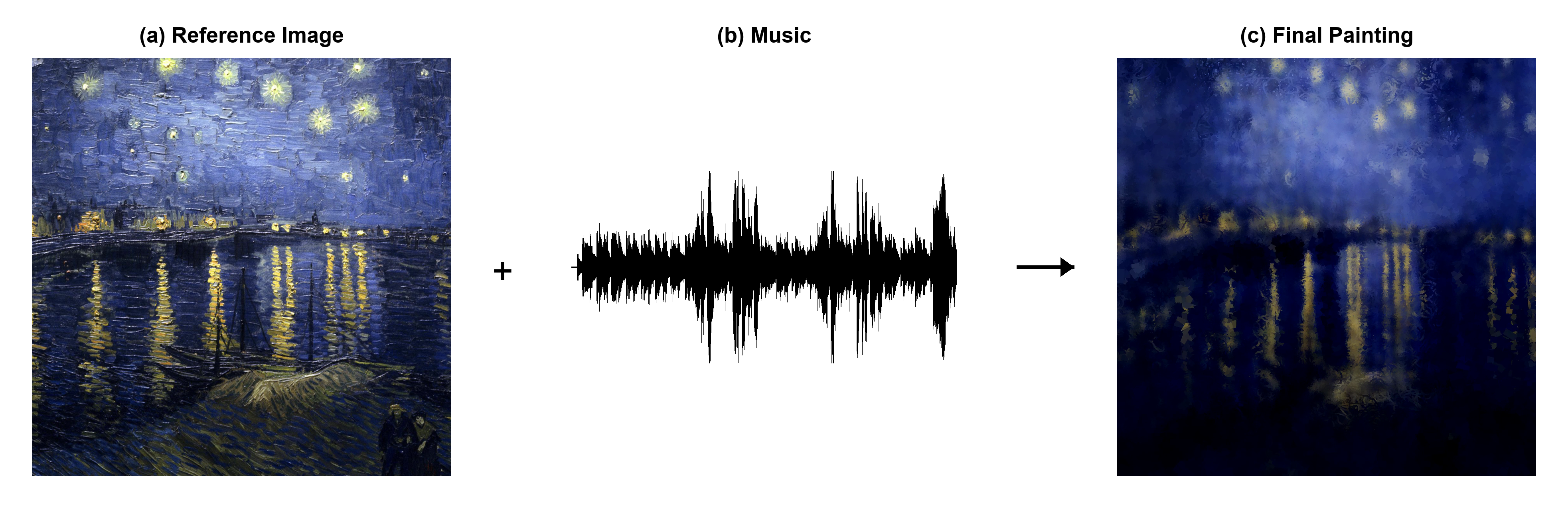
Figure 1. The basic artistic problem in Inner Landscapes, shown with a Grief example: combine a reference image with music to create frames of a final moving painting. This figure shows the goal before we study the technical pieces that make it possible.
Figure 1 shows the project at the level of an artist’s question. We begin with something visual and something musical, and we want the final result to feel like both of them at once. The rest of the chapter explains how the computer builds that connection step by step.
A useful starting point is NeuroMV: A Neural Music Visualizer, described by Kayo Yin and collaborators in 2022. NeuroMV represents music with a Mel spectrogram and samples music features at video-frame speed. For each frame, it gives a neural network two kinds of information: an image location and the current music features. The network then predicts an RGB color. This matters for our project because it shows a simple but powerful idea: music can become part of the input to an image-making rule.
Inner Landscapes uses that idea as a foundation, but not as the whole method. The neural network supplies predicted color, while the random walk supplies marks and movement. Later sections explain the training process, zoom targets, image-region information, and rendering steps in detail. For now, the important point is that the project needs both a learned color rule and a way to turn that rule into a painting over time.
A neural network is a computer model that learns from examples. At first, it does not know the right colors for the image. During training, it makes guesses, compares those guesses with target colors, and adjusts itself so that future guesses become closer. In this chapter, the neural network learns a color rule: given an image location and the current music features, predict an RGB color.
However, predicting colors is not the same as making a painting. A painting also needs marks, movement, and time. For that part, we use a random walk. A random walk is a path made from many small steps. Each step continues from the current position, but its direction can change. In Inner Landscapes, many virtual walkers move across the canvas. As they move, they leave colored strokes behind them. The neural network chooses the stroke color, while the music and image-region information help control how the walkers move and how visible their strokes are.
Key Distinction: The neural network does not draw the path. It predicts a color from an image location and current music features. The random walk creates the path of marks across the canvas. Together, they turn color prediction into a moving painting.
The challenge is that a computer cannot begin with a feeling such as calm or nostalgia. It needs a clear sequence of numerical steps. We must turn music into numbers, connect those numbers to image locations, train a neural network, and then use random walks to draw the final frames. The next section gives the complete map of this system.
Methodology
Overall Methodology
The question we need to answer is: how do we turn a still reference image and a changing piece of music into a painting that changes over time? At the conceptual level, the workflow is:
reference image + music -> music representation and zoom targets -> train neural network -> random-walk painting -> saved frames -> final video.
The first part of the pipeline happens during training. The program loads a reference image and an audio file for one emotion. It converts the audio into music features and also uses the music to choose one of three zoomed versions of the reference image. These zoomed versions are called zoom targets. They represent three visual scales of the same image.
The neural network is trained from these examples. During each training step, the program chooses one sampled music frame. The music features from that frame are paired with every image location on a training grid. The neural network predicts a color for each location. The predicted colors are compared with the colors in the selected zoom target. By repeating this process, the neural network learns a rule that connects image location, music features, and predicted color.
When training is finished, the program saves a checkpoint. A checkpoint is not a separate artistic stage. It is an implementation bridge between training and rendering: a file that stores what the neural network learned, along with important settings such as the spectrogram normalization values, image size, music frame rate, zoom levels, and zoom crop sizes. The notebook later loads this checkpoint instead of training the model again.
The second part of the pipeline happens during rendering. The notebook chooses an audio segment, rebuilds the music features for that segment, loads the trained neural network from the checkpoint, and creates a random-walk painter. The painter starts with a blank canvas. At each frame, each walker takes many small steps. At each walker location, the neural network uses the current image location and current music features to predict the stroke color. The music also affects the walker movement and stroke appearance. Image-region information derived from the reference image lets different parts of the canvas behave differently.
The canvas is saved many times as a sequence of still images, called frames. These frames are then combined with the music to create the final video.
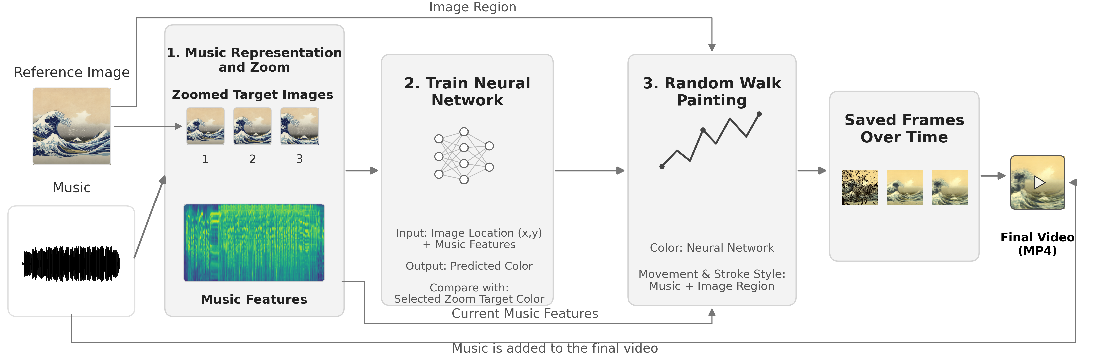
Figure 2. Overview of the Inner Landscapes workflow. Music features and zoomed target images are used to train a neural network to predict image colors. During painting, the trained network uses current music features to predict stroke colors, while music and image-region information guide the random-walk movement and stroke style. The saved frames and music are finally combined into a video.
Figure 2 gives us a simple map of the process. We can now begin with the first stage: what does music look like to a computer, and how can it be used to control visual scale?
Music Representation and Zoom
From Sound to a Mel Spectrogram
Before the computer can use music, the sound must first be stored as numbers. A digital audio file does this by recording many measurements over time. Each measurement is called a sample. The sample rate tells us how many samples are stored in one second. In the main emotion audio files for this project, the sample rate is samples per second.
The samples describe the shape of the sound wave, but the project needs more than the wave shape. It also needs to know which frequencies are present. Frequency describes how quickly a vibration repeats. Low frequencies usually sound deeper. High frequencies usually sound higher. Music contains many frequencies at the same time, and these frequencies change as the music plays.
To see these changes, we do not analyze the entire song at once. Instead, we examine many short sections of the audio called windows. For each window, frequency analysis measures how strongly different frequencies are present. Then the window moves forward and the process repeats. This gives the computer a new description of the music many times per second.
Placing the results from all of these windows next to one another creates a spectrogram. The horizontal direction represents time, the vertical direction represents frequency, and the value at each location shows how strongly that frequency is present at that moment. In this way, a spectrogram lets us see both when something happens and which frequencies are present.
Our program uses a target rate of music frames per second. This matches the video frame rate used later. If the audio has a sample rate of samples per second, the distance between two neighboring music frames is
where is called the hop length. The floor brackets mean that the program keeps the whole-number part of the result because it must move by a whole number of samples.
For the main emotion audio files,
so
Neighboring music frames are therefore spaced samples apart. The program analyzes a window that is twice this length, or samples. Because the window is wider than the distance between neighboring frames, neighboring windows overlap.
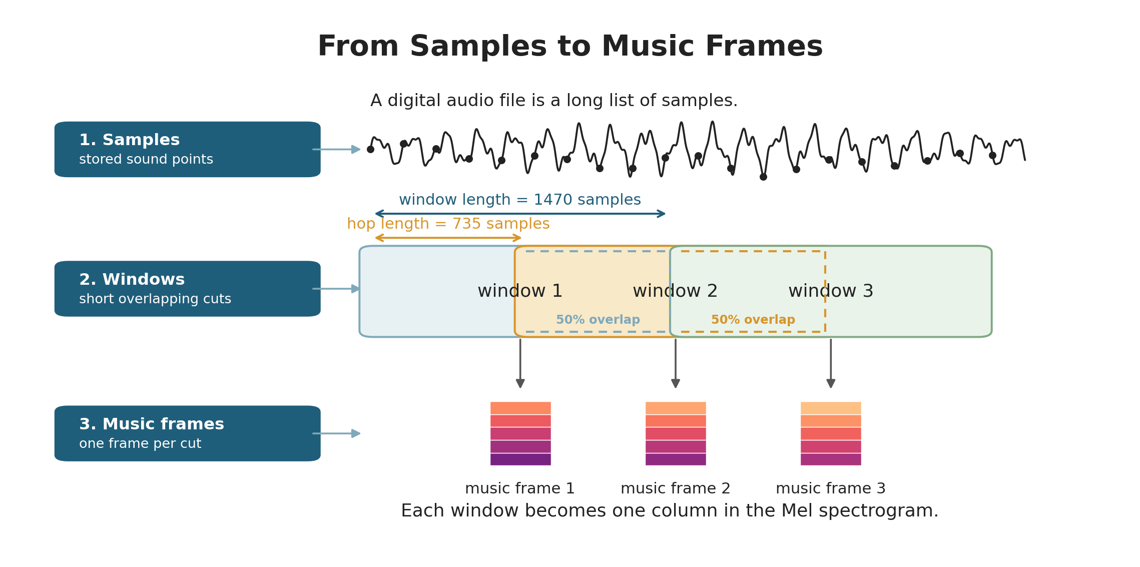
Figure 3. A sound wave is stored as samples. The program analyzes overlapping windows of samples. Each new window begins one hop length after the previous one, and each window becomes one music frame for the Mel spectrogram.
Figure 3 shows why the hop length matters. The program is not listening to one isolated instant. It is looking at a short window of sound, then sliding that window forward. This gives the system a steady stream of music frames that can be aligned with video frames.
A regular spectrogram organizes the result using frequency. Our system uses a Mel spectrogram. A Mel spectrogram groups frequencies into bands called Mel bins. These bands are arranged on a scale that roughly follows how people perceive differences between lower and higher sounds. The result is still organized by time and frequency, but each time frame is now represented by a list of Mel values.
The project uses two Mel spectrogram settings. For the neural network, each music frame has Mel values. This means one frame of music becomes a vector with shape . Across the whole audio file, the spectrogram has shape , where is the number of music frames. For zoom decisions, the program also computes a second Mel spectrogram with Mel bins. That second representation is used later to decide which zoom target should be selected.
Useful Rule: The -bin Mel spectrogram provides music features for predicted color. The -bin Mel spectrogram helps choose visual scale. They both come from the same sound, but they serve different jobs in the system.
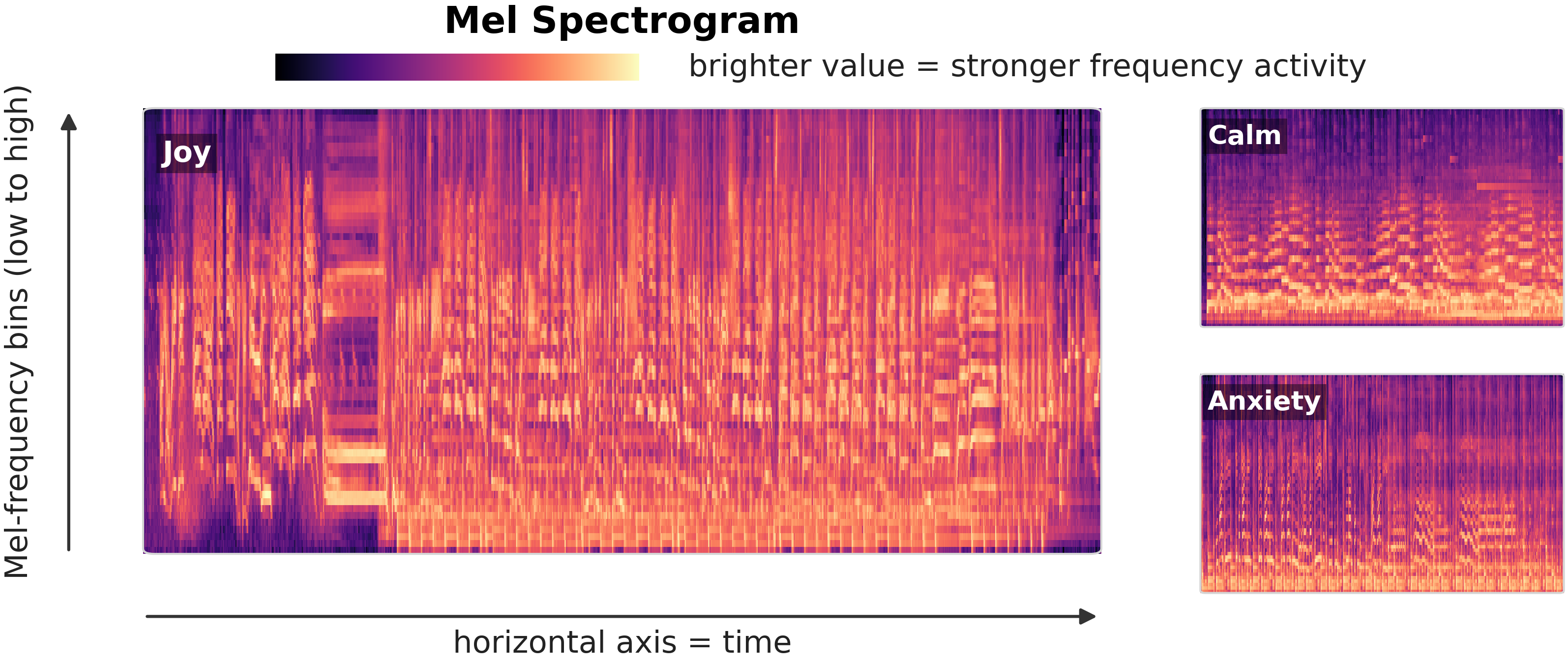
Figure 4. Mel spectrogram examples from the Joy, Calm, and Anxiety pieces.
Figure 4 shows Mel spectrograms from three pieces in Inner Landscapes. The horizontal axis represents time, while the vertical axis represents Mel frequency bins. Brighter regions show stronger activity in those frequency bands. The different patterns in the Joy, Calm, and Anxiety examples show how different pieces of music produce different distributions of frequency activity over time.
Now that we know how sound becomes a Mel spectrogram, we can look at the first job of that representation: providing music features to the neural network.
Music Features for the Neural Network
The Mel spectrogram gives us a new description of the music at many moments in time. The next question is how the neural network can use one of those moments. A single music frame tells the computer what the music is doing now. It does not tell the computer where in the image a color should be predicted. For that reason, the music features must be paired with an image location.
Let represent the -bin Mel vector at time frame . After the log transform and normalization, each entry of this vector is scaled to the range from to . This vector is the current music features. It gives a compact numerical summary of the sound at that moment.
The neural network does not receive alone. It receives together with a location from the image grid. The model’s question is local: given an image location and the current music features, what RGB color should appear here?
During training, the image is represented on a grid, so one full grid contains image locations. For one selected music frame, the same music values are repeated for every location on this grid. Each row of the model input contains two coordinate values and music values:
Therefore, one training input for one music frame has shape . The columns come from coordinate values plus music values.
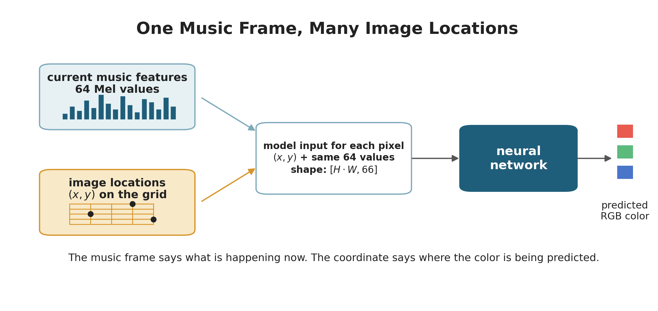
Figure 5. One music frame is paired with many image locations. The same current music features are repeated across the image grid, so the neural network can predict a separate RGB color at each location.
Figure 5 shows the main idea. The music frame describes the current sound. The image location tells the network where it is being asked to predict a color. The output is not a whole image all at once in the usual sense. It is a color rule applied many times, once for each location.
Key Distinction: The music features describe time. The image location describes space. The neural network needs both: without music, the color would not respond to the song; without location, the model would not know where in the image the color belongs.
The target color for each location comes from a version of the reference image. Which version is used depends on the selected zoom target. That is the second job of the music representation.
Music-Driven Zoom
Music does more than provide color features. It also helps decide the visual scale of the target image. A calm or quiet moment may use a wider view of the reference image. A stronger moment may use a closer view. This gives the system a way to connect musical change with visual zoom.
The program uses a second Mel spectrogram for this purpose. The color model uses Mel bins, but the zoom decision uses Mel bins. For each time frame, the program looks at the th percentile of the normalized log-Mel values:
where is the -bin Mel vector at time frame after log scaling and normalization. The value is not the loudness of the whole song. It is a high-energy summary of one music frame. It asks: how strong are the stronger frequency bands right now?
The raw signal can jump too quickly from frame to frame, so the program smooths it with a moving average. It then normalizes the smoothed signal again and compares it with two emotion-specific threshold values. These thresholds divide the signal into three zoom levels:
Here is the lower threshold and is the higher threshold. In the source code, these levels are stored as , , and , but in the explanation we call them level , level , and level because that is easier to read.
The threshold values are not the same for every emotion. The program chooses them from percentiles of that emotion’s own signal. This matters because a quiet piece and an intense piece can have very different numerical ranges. Percentile thresholds let each piece use the three zoom levels in a way that fits its own music.
The program also uses two stabilizing ideas. First, a zoom level must last for a minimum amount of time before it can change again. Second, a small hysteresis margin prevents the level from flickering when the signal sits close to a threshold. Hysteresis means that the signal must move a little past the threshold before the level changes back. These choices make the visual scale change more smoothly.
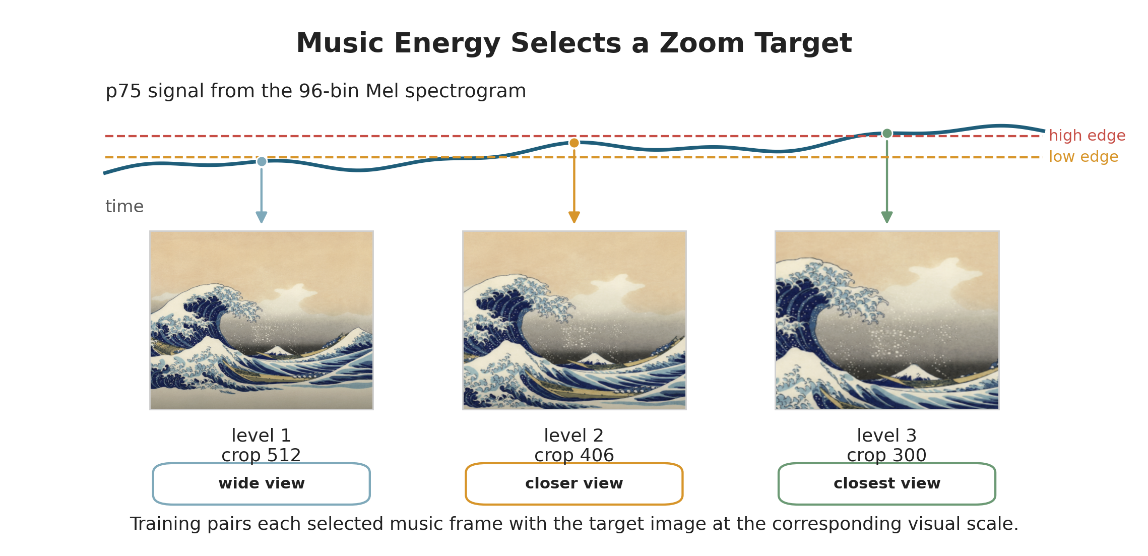
Figure 6. A smoothed music-energy signal is divided by low and high thresholds into three visual scale levels. Smaller crop sizes create stronger zoom targets. The Joy example uses crop sizes , , and .
Figure 6 shows the result for the Joy reference image. Level uses the widest view. Level crops the image more tightly and resizes it back to the training size. Level uses the smallest crop, so it looks closest. The neural network then learns colors from the zoom target selected for the sampled music frame.
The crop sizes are not the same for every emotion. Each piece has its own visual scale settings:
| Emotion | Zoom crop sizes |
|---|---|
| calm | 486, 423, 360 |
| nostalgia | 512, 451, 390 |
| grief | 512, 426, 340 |
| joy | 512, 406, 300 |
| anxiety | 512, 426, 340 |
Useful Rule: A smaller crop size means a stronger zoom. The image is cropped around the center and then resized back to the training grid, so the neural network always predicts colors on the same coordinate system.
The training program samples music frames from the available zoom levels, so the model sees examples from each visual scale. This prepares the neural network to connect current music features, image location, and selected zoom target. The next section explains what kind of neural network can learn that connection.
Neural Image Representation
The reference image begins as pixels, but the trained system does not simply copy those pixels into the final video. Instead, it learns a coordinate-based image rule. The rule takes an image location and current music features as input, then returns a predicted RGB color.
What the Neural Network Learns
A neural network is a function with many adjustable numbers inside it. These adjustable numbers are called weights and biases. At the start of training, they do not yet describe the reference image well. Training changes them until the network gives better color predictions.
In this project, the network is not asked to classify an image or name an emotion. Its job is more direct. For a location and current music features , it predicts an RGB color:
The symbol means “the color predicted by the network.” The hat reminds us that this color is a prediction. The symbol stands for all the learned weights and biases inside the network. The output has three numbers because an RGB color has a red value, a green value, and a blue value. The final layer uses a sigmoid function, so these three numbers stay between and .
This is useful because a rule can be queried at any location. During training, the locations come from the grid. During rendering, the random walkers visit locations on a larger canvas, and those locations are normalized before being sent to the same learned rule.
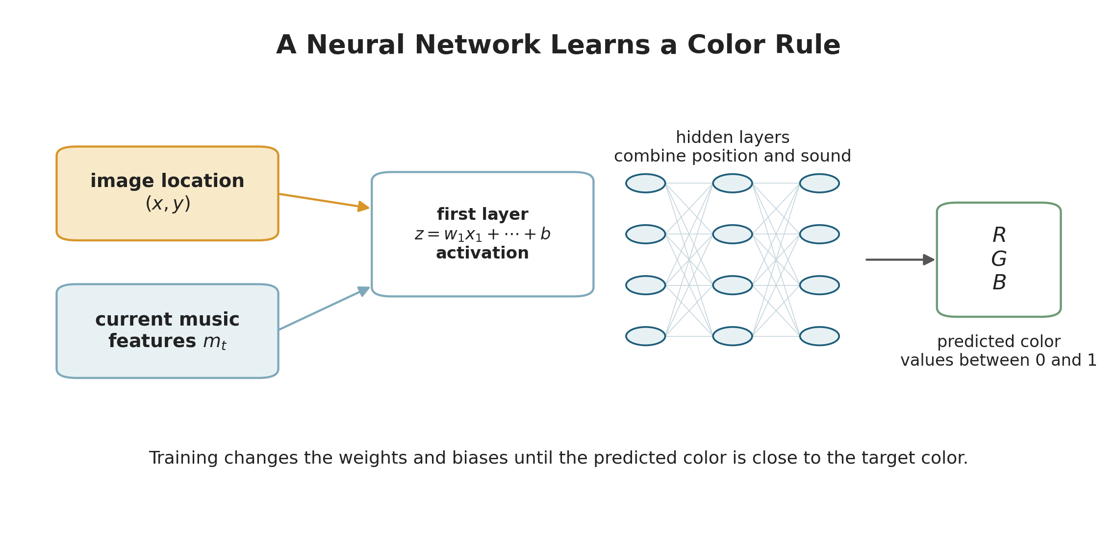
Figure 7. The neural network learns a color rule. It receives an image location and current music features, passes them through learned layers, and outputs a predicted RGB color.
Figure 7 shows the network as a chain of transformations. The input gives the network a question. The hidden layers transform that question into intermediate values. The output gives the predicted color.
Neurons, Layers, and Activations
The basic unit of a neural network is a neuron. A neuron takes several input numbers, multiplies each one by a weight, adds a bias, and produces a new number. In a simple case, this looks like
Here are input values, are weights, and is the bias. If a weight is large, that input has a stronger effect on the neuron. If a weight is close to zero, that input has little effect.
After computing , the network applies an activation function. An activation function bends the number before sending it to the next layer. The hidden layers in this project use the hyperbolic tangent function, written as . Without activation functions, stacking many layers would still behave like one large linear calculation. With activation functions, the network can learn curved and detailed relationships, such as how color changes across waves, clouds, sky, or water.
A layer is a group of neurons working side by side. This project uses several hidden layers, each with neurons. The first layer receives the encoded image location and the music features. Later layers combine these values into more useful internal patterns. The final layer produces the three RGB numbers.
Concept in Focus: A neural network is not magic memory. It is a large adjustable formula. Training changes the weights and biases so that the formula maps image location and current music features to a useful predicted color.
The Forward Pass
The calculation that goes from input to output is called the forward pass. First, the program builds one input vector from the encoded location and the current music features. Then each layer transforms the vector it receives:
and the same pattern continues through the hidden layers. Here and are matrices of weights, and and are bias vectors. A matrix is just a rectangular table of numbers. Multiplying by the matrix lets one layer combine many input values at once.
After the hidden layers, the final layer produces three output values:
The symbol is the sigmoid function. It squeezes each output value into the range from to , which matches the normalized RGB color range used during training. This is why the network can be trained with image colors as targets.
Fourier Features for Image Location
The first part of the input is the location . The program normalizes each coordinate so that the image ranges from to in both directions. A normalized coordinate system makes the model less dependent on the raw pixel size of the canvas. The left side of the image is near , the right side is near , and the top and bottom are represented in the same way along the direction.
The coordinate is then expanded with sine and cosine features. This is called a Fourier-style coordinate encoding. The purpose is to give the network several ways to sense position: broad, slow changes and smaller, faster changes. The standard implementation uses the frequencies
The Nostalgia model uses one additional frequency, , but the idea is the same. The extra frequency gives that model one more fine-scale coordinate pattern.
These encoded coordinates help the network represent image detail more easily than raw alone. Raw coordinates change smoothly from left to right and top to bottom. That smoothness is useful, but it can make fine visual structure harder to learn. Sine and cosine features add repeating patterns at several scales, giving the network more ways to describe edges, waves, and small changes in the image.
For each frequency, the program adds sine and cosine versions of both coordinates. In the standard setting, the two raw coordinate values therefore become
coordinate features. With the extra Nostalgia frequency, the coordinate part becomes features. In both cases, these coordinate features are then combined with the music features inside the network.
L1 and L2 Color Loss
Training needs a way to tell whether the predicted color is good. For a sampled music frame , the program already knows the selected zoom target. At each location, the model predicts a color, and the program compares that prediction with the color from the selected zoom target:
The loss is one number that summarizes how wrong the prediction is. The program combines two common kinds of color error: L1 loss and L2 loss.
L1 loss measures absolute difference:
This means it looks directly at the size of the color mistake. If the prediction is off by , the L1 error is . If it is off by , the L1 error is . L1 loss is useful because it is not dominated too strongly by a few very large mistakes. In image problems, this can help preserve sharper structure.
L2 loss measures squared difference:
Squaring makes larger mistakes count more. An error of becomes , while an error of becomes . This encourages the model to reduce large color errors and often gives smoother training behavior.
Inner Landscapes uses both:
The two terms have equal weight. The L1 part keeps the model from caring only about large errors, while the L2 part still pushes the network to correct large mistakes. Together, they give a balanced color-learning signal.
Edge-Weighted Training
The program also gives different image locations different weights. The weight map is built from edge strength in the reference image, with a base weight so that non-edge pixels still matter. This helps the model pay more attention to visually important structure without completely ignoring smoother regions.
This matters because not every pixel has the same visual importance. A small color error along the outline of a wave may be more noticeable than the same size error in a smooth region of sky. Edge-weighted training tells the model, in effect, to spend extra attention on locations where the reference image has stronger structure.
If is the image weight at one location, the local training loss can be understood as
The full loss is the average of this weighted error over sampled locations, color channels, and training examples.
Backpropagation and the Checkpoint
Once the loss is computed, the network must know how to change its weights. This is where derivatives enter. A derivative tells us how much one number changes when another number changes. If a small increase in one weight makes the loss larger, training should push that weight downward. If a small increase makes the loss smaller, training may push that weight upward.
Backpropagation is the method that computes these directions for all the weights. It starts from the output error and moves backward through the network. For a simple chain, the idea is the chain rule:
This equation says that a weight affects the loss through the later values it helps create. The real network has many layers and many weights, but the principle is the same. PyTorch performs this derivative calculation automatically. Then the Adam optimizer updates the weights in small steps. The learning rate in the training script is , so the updates are careful rather than sudden.
Concept in Focus: The checkpoint does not store the finished painting. It stores the trained color rule, normalization values, image size, music frame rate, Fourier frequencies, zoom levels, and zoom target information needed to rebuild the system later.
This section gives the central neural representation: an image is treated as a learned function from location and music to color. The next section explains how that color function becomes visible as strokes on a canvas.
Audio-Driven Random Walk Painting
From Color Rule to Moving Strokes
The neural network can predict colors, but it does not decide where to draw. The moving painting needs a path. In Inner Landscapes, that path is created by random walkers.
A random walker has a current position and a current direction. We can write its state at step as
where is the walker’s position and is the direction angle. At each small step, the direction changes by a random amount. In the code, this random turn is sampled from a normal distribution:
so the new direction is approximately
The walker then moves forward using basic trigonometry:
where is the step length. This is the essential mathematics of the random walk used here: turn a little, move forward, repeat. If the next position reaches the boundary of the canvas, the direction is reflected back into the image. This keeps the walker inside the painting area. The walkers do not begin from one single point. They are initialized across a grid of canvas cells, so the painting can start building in many regions.
The notebook does not train the model again. It loads the checkpoint, rebuilds the neural network, restores the saved weights, cuts the chosen audio segment, and recomputes the music features for that segment using the same normalization values saved during training. Then it creates an RW_Painter.
At frame , the painter takes the current music features . The model uses these features for color prediction. The painter also computes a simple music intensity value:
This intensity value controls how active the walkers become. A stronger frame produces longer steps, thicker strokes, larger turning variation, and higher opacity. In simplified form, the base controls are
Emotion-specific parameters then scale these quantities. For example, a piece can use more walkers, larger step scale, stronger turning scale, or a different color tint. These choices affect the visual style of the piece without changing the basic rule: music features and image location still determine the predicted color.
Key Distinction: Music features have two jobs during rendering. The full current music vector is used by the neural network to predict color. The single intensity value from that vector is used by the painter to control motion and stroke appearance.
Image-Region Information and Local Style
The painter also uses image-region information from the reference image. This information does not replace the neural network. It affects how the walkers move and how strongly they draw in different parts of the canvas.
The program first converts the reference image to grayscale and measures edge strength with image gradients. Then it selects lower-edge regions, blurs that selection, and turns the result into a region weight between and . During rendering, the active region map is matched to the current zoom level, so the region guidance follows the same visual scale as the selected zoom target.
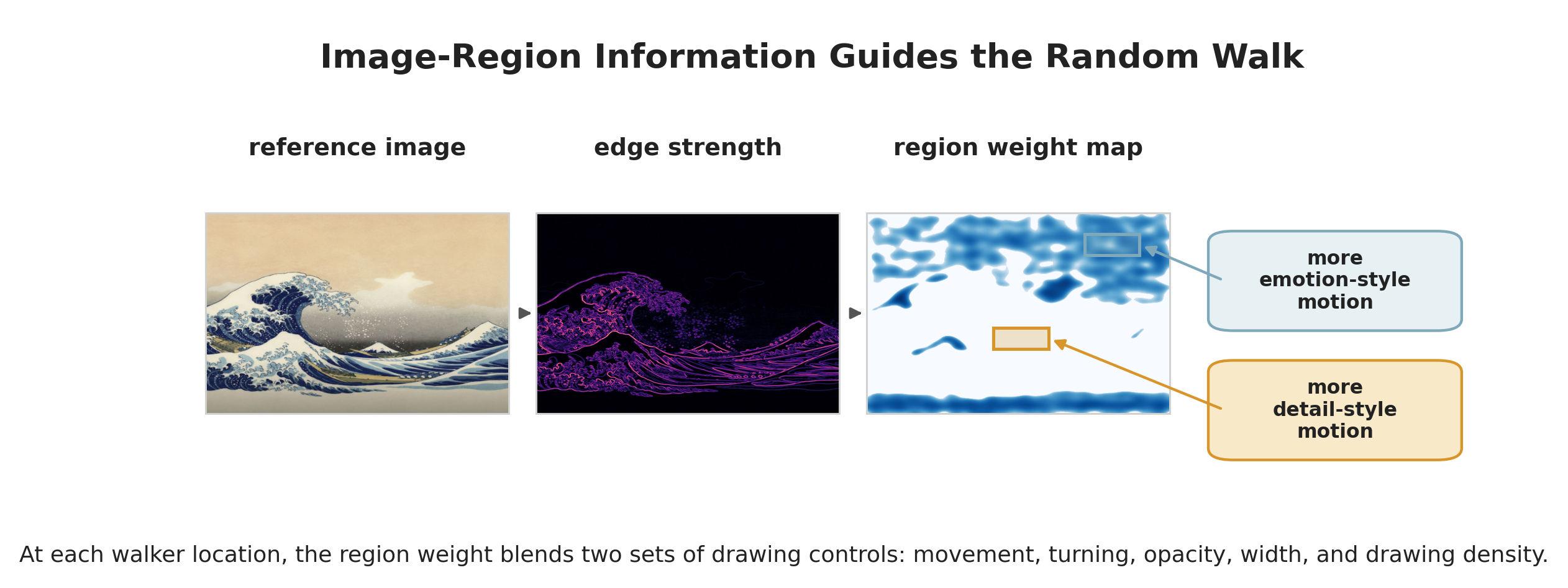
Figure 8. Image-region information guides local random-walk behavior. The reference image is converted into edge strength and then into a region weight map. Blue high-weight regions favor emotion-style controls, while pale low-weight regions favor detail-style controls.
Figure 8 shows why the region map is useful. Some locations use more emotion-style behavior, which can mean stronger movement, opacity, width, or drawing density. Other locations use more detail-style behavior, which is usually softer and more controlled. The final stroke parameters are blended from these two behaviors at the walker’s current location.
The blend is a simple weighted average. If is the region weight at the current walker location, then a local control value can be written as
Here can stand for step length, turn variation, opacity, stroke width, or the number of drawing steps used in one frame. When is close to , the emotion-style control dominates. When it is close to , the detail-style control dominates. Values between and smoothly mix the two.
Each walker step follows the same basic sequence:
choose local drawing controls -> turn -> move -> predict color -> draw a stroke.
The canvas is not cleared between frames. Each new stroke is added on top of the previous strokes. This is why the result feels like a painting being built over time rather than a set of unrelated images.
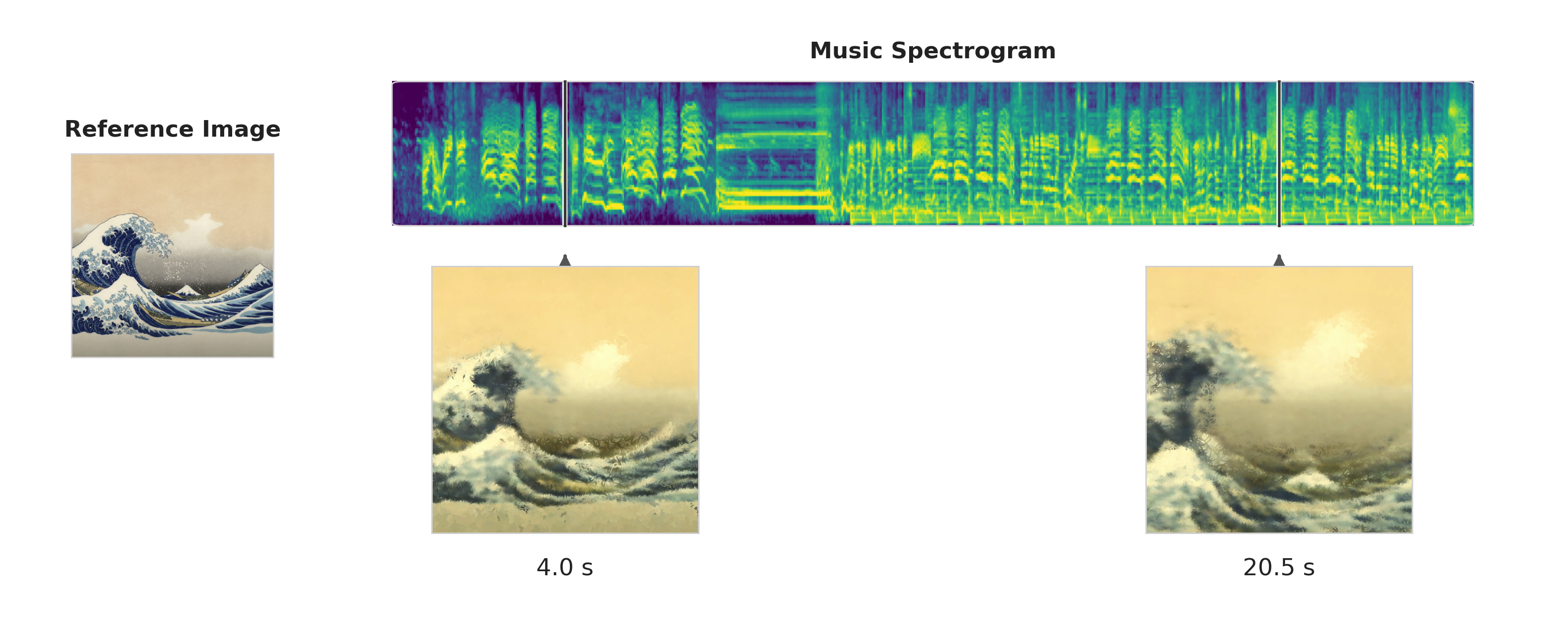
Figure 9. Two moments from a Joy rendering. The current music features come from different time positions in the spectrogram, and the accumulated random-walk painting looks different at those moments.
Figure 9 shows this time-based behavior. The reference image gives the visual world, the spectrogram gives changing music features, and the random walkers turn those features into accumulated marks. After the painter saves all frames, the frames are combined with the audio to create the final video.
Program
The Methodology section explained the ideas. This section connects those ideas to the actual program. The goal is not to memorize every line of code. The goal is to know where each part of the system happens and how data moves from one file to the next.
The code is organized around three main files:
| File | Main job |
|---|---|
neural_network_music.py | train the neural color model and save checkpoints |
random_walk_image.ipynb | load checkpoints, choose audio clips, and start rendering |
RWraw.py | run the random-walk painter and save frames |
The real implementation follows the engineering workflow introduced earlier:
training -> checkpoint -> notebook integration -> RW_Painter rendering -> frames -> final video.
This is the code-level version of the conceptual workflow. The conceptual workflow tells us what the system means. The code workflow tells us where the files hand information to one another.
Training the Neural Color Model
Training happens in neural_network_music.py. This file contains the audio-feature functions, the zoom-level functions, the neural network class, the training loop, and the checkpoint-saving step.
The training jobs are stored in a dictionary. Each job gives the program the main files and settings needed for one emotion:
TRAINING_JOBS = {
    "joy": {
        "image": "joy.png",
        "audio": "Joy.wav",
        "ckpt": "ckpts/joy_ckpt.pt",
        "zoom_crop_sizes": EMOTION_ZOOM_CROP_SIZES["joy"],
    },
}
The full dictionary includes the five emotions used by the project. The important idea is that the same training function can be reused. The program changes the image, audio, checkpoint path, and settings for each emotion, but the basic training procedure stays the same.
At the bottom of the file, the script loops over the training jobs:
for emotion_name, cfg in TRAINING_JOBS.items():
    train_emotion_model(
        emotion_name=emotion_name,
        image_file=cfg["image"],
        audio_file=cfg["audio"],
        ckpt_path=cfg["ckpt"],
        emotion_zoom_crop_sizes=cfg["zoom_crop_sizes"],
        emotion_fourier_frequencies=cfg.get("fourier_frequencies"),
    )
This loop is the start of the training pipeline. For each emotion, it calls train_emotion_model. That function prepares the image, prepares the music, trains the model, and saves the checkpoint.
Building Training Examples
Inside train_emotion_model, the first major task is to turn the image and audio into training examples. The image is resized to the training grid:
H, W = 512, 512
target_img = Image.open(image_file).convert("RGB").resize((W, H))
The program also creates one coordinate for every pixel location. These coordinates are normalized from to , matching the coordinate system explained in the Methodology section.
Next, the audio becomes music features:
raw_spec = make_mel_spec(audio_file, latent_size, target_fps)
spectrogram, spec_min, spec_max = normalize_spec(raw_spec)
The first line builds the -bin Mel spectrogram. The second line applies the log transform and normalization. The values spec_min and spec_max are saved because the notebook must normalize later audio clips in the same way.
The program also computes zoom levels from a separate -bin Mel spectrogram:
raw_zoom_spec = make_mel_spec(audio_file, p75_zoom_mels, target_fps)
p75_signal, zoom_levels, edges, percentiles = compute_p75_zoom_levels(
    raw_zoom_spec, emotion_name, target_fps
)
The result zoom_levels tells the training code which zoom target should be used at each music frame. A frame with a lower zoom level uses a wider target image. A frame with a higher zoom level uses a closer target image.
When the model trains on one music frame, the same music vector is repeated for every image location:
music_vec = spec_frame.unsqueeze(0).repeat(H * W, 1)
inp_train = torch.cat([coords, music_vec], dim=1)
This creates the input table described earlier. Each row contains one image location and the current music features. The network can then predict one RGB color for each row.
Training Loop and Loss
The neural network itself is defined by the class XYSpecNet. Its input is the pair of ideas we have been using throughout the chapter: image location and current music features. Its output is a predicted RGB color.
During training, the program repeatedly chooses a sampled music frame, builds the model input, predicts colors, computes the loss, and updates the weights:
pred = model(inp_train)
l1 = torch.abs(pred - target_music_tensor)
l2 = (pred - target_music_tensor) ** 2
loss = ((0.5 * l1 + 0.5 * l2) * pixel_weights).mean()

loss.backward()
optimizer.step()
These lines are the code version of the loss and backpropagation discussion. The prediction pred is compared with target_music_tensor, which contains the target RGB colors from the selected zoom image. The L1 and L2 terms measure color error. The pixel_weights term gives extra importance to image locations with stronger edge structure.
The line loss.backward() asks PyTorch to compute the derivatives. The line optimizer.step() uses those derivatives to update the weights. In this project, the optimizer is Adam with learning rate .
Practical Takeaway: The training script does not paint the final video. It teaches a neural network to answer one question well: given an image location and current music features, what color should be predicted?
Saving the Checkpoint
After training, the script saves a checkpoint. A checkpoint is the handoff from training to rendering. It stores the trained model weights and the settings needed to rebuild the same model later.
A shortened version of the checkpoint code looks like this:
torch.save(
    {
        "model_state_dict": model.state_dict(),
        "spec_min": spec_min,
        "spec_max": spec_max,
        "zoom_levels": zoom_levels,
        "zoom_crop_sizes": emotion_zoom_crop_sizes,
    },
    ckpt_path,
)
The real checkpoint stores more fields, including image size, music frame rate, hidden-layer size, Fourier frequencies, loss history, and paths to visual checks. The most important field is model_state_dict. It contains the learned weights and biases of the neural network.
The checkpoint is why the rendering notebook does not have to train again. It can rebuild the model, load the saved weights, and continue from the trained color rule.
Notebook Integration
Rendering begins in random_walk_image.ipynb. The notebook imports the trained model class and helper functions from neural_network_music.py, and it imports the painter from RWraw.py:
from neural_network_music import XYSpecNet, make_mel_spec, normalize_spec
from neural_network_music import frames_to_video_with_audio
from RWraw import RW_Painter
The notebook then loads one checkpoint:
ckpt = torch.load(ckpt_file, map_location="cpu")
latent_size = ckpt["latent_size"]
hidden = ckpt["hidden"]
target_fps = ckpt["target_fps"]
These values tell the notebook how to rebuild the network. The model must have the same input dimension, hidden size, and Fourier encoding that were used during training.
The notebook rebuilds the neural network and restores its learned weights:
model = XYSpecNet(
    spec_dim=input_spec_dim,
    hidden=hidden,
    fourier_frequencies=model_fourier_frequencies,
)
model.load_state_dict(ckpt["model_state_dict"])
model.eval()
The call to model.eval() puts the model in evaluation mode. In simple terms, the model is no longer learning. It is now being used to make predictions.
The notebook also cuts the selected audio segment and recomputes the music features for that segment:
make_audio_clip(audio_file, start_sec, end_sec, clip_file)
raw_spec = make_mel_spec(clip_file, latent_size, target_fps)
spec, _, _ = normalize_spec(raw_spec, spec_min=spec_min, spec_max=spec_max)
Notice that the same spec_min and spec_max from training are reused. This keeps the meaning of the music-feature values consistent between training and rendering.
The notebook also slices the saved zoom levels so that the zoom behavior lines up with the chosen audio clip:
zoom_start_frame = int(round(start_sec * target_fps))
zoom_levels = full_zoom_levels[
    zoom_start_frame:zoom_start_frame + num_frames
]
This step matters because rendering may use only part of the original audio file. The zoom levels must start at the same musical time as the clip.
RW Painter Rendering
The notebook creates an RW_Painter. This object owns the canvas, the walker positions, the walker directions, the image-region map, and the drawing process:
painter = RW_Painter(
    model, W_RENDER, H_RENDER,
    num_walkers=cfg["num_walkers"],
    emotion_params=emotion_params,
)
The model gives the painter a way to predict color. The render size gives the painter the canvas size. The walker count and emotion parameters control how many walkers move and how their strokes behave.
Then the notebook starts rendering:
painter.render(
    spec=spec,
    num_frames=num_frames,
    steps_per_frame=cfg["steps_per_frame"],
    output_dir=output_dir,
    target_fps=target_fps,
    zoom_levels=zoom_levels,
)
Inside RWraw.py, the render method loops over the frames. For each frame, it selects the current music features, chooses the active zoom-level region map, computes music intensity, updates every walker, predicts stroke colors with the neural network, and draws lines onto the accumulating canvas.
Each saved frame is named with six digits:
frame_path = os.path.join(output_dir, f"{f:06d}.png")
self.canvas.save(frame_path)
This naming pattern is important because video tools expect frames to be in a clean numerical sequence, such as 000000.png, 000001.png, and 000002.png.
Frames and Final Video
The last step is handled by frames_to_video_with_audio. The notebook calls it after all frames have been rendered:
frames_to_video_with_audio(
    output_dir=output_dir,
    output_name=output_name,
    audio_file=clip_file,
    target_fps=target_fps,
)
This helper function uses ffmpeg twice. First, it turns the numbered PNG frames into an MP4 video. Then it adds the audio clip to that video. The final result is a video file whose images and audio share the same frame rate and duration.
Useful Rule: In the code, training and rendering are separate.
neural_network_music.pylearns and saves the color rule.random_walk_image.ipynbreloads that rule.RWraw.pyturns the reloaded rule into painted frames.
Exercises
These exercises are meant to check understanding of the full chapter. Some questions ask for short explanations. Others ask for small calculations using the numbers already introduced. None of them require writing a full neural-network program.
Sound and Music Features
- In one or two sentences, explain why the program converts sound into a Mel spectrogram instead of using the raw audio wave directly.
- The project uses a target rate of music frames per second. If an audio file has sample rate , calculate the hop length.
- If one music frame has Mel values, what is the shape of a spectrogram with music frames?
- Explain the difference between the -bin Mel spectrogram and the -bin Mel spectrogram in this project.
- Why does the program use a log transform and normalization before giving music features to the neural network?
- In your own words, explain why a single music frame must be paired with image locations before it can be used for color prediction.
Neural Network and Training
- During training, the image grid has size . How many image locations are in one full grid?
- One model input row contains and music values. How many input values are in that row before Fourier coordinate encoding?
- Explain what a weight and a bias do inside a neuron.
- Why does the network use activation functions between linear layers?
- Write the meaning of the expression in words.
- Suppose a predicted color channel is and the target color channel is . Compute the L1 error, the L2 error, and the combined error for that one channel.
- Why does the training loss use both L1 and L2 error instead of only one of them?
- Explain why edge-weighted training gives extra attention to visually important parts of the reference image.
- What is backpropagation used for during training?
- Name three kinds of information saved in the checkpoint.
Zoom and Random-Walk Rendering
- What does a smaller zoom crop size mean visually?
- Explain why the program uses percentile thresholds instead of one fixed numerical threshold for every emotion.
- A random walker has state . What does each part of this state represent?
- If a walker starts at , has direction , and takes a step of length , what is its new position before any boundary reflection?
- If the current music intensity increases, what happens to step length, stroke width, turn variation, and opacity?
- A local drawing control is computed as . If , , and , compute .
- Why is the canvas not cleared between frames?
Program Workflow
- Put these stages in the correct order: notebook integration, final video, training,
RW_Painterrendering, checkpoint, frames. - Which source file defines
XYSpecNet? - Which source file defines
RW_Painter? - Which file loads the checkpoint and starts the rendering process?
- If an audio clip lasts seconds and the target frame rate is frames per second, about how many frames should be rendered?
- Why does the notebook reuse
spec_minandspec_maxfrom the checkpoint when it normalizes the rendering audio clip? - What does
frames_to_video_with_audiodo after all PNG frames have been saved?
Results
The final output of the project is a video, but a still frame is a useful way to study what the system has produced. A finished frame shows the accumulated canvas after many random-walk strokes have already been drawn. By this point, the frame contains information from the reference image, the trained neural color rule, the selected zoom targets, and the changing music features.
Figure 10 shows one late frame from each final video. These frames should not be read as five isolated pictures. They are snapshots from moving paintings. The visible result at any moment depends on what the music has done up to that time and how the canvas has accumulated previous strokes.
How to Read the Output
When looking at the results, it helps to ask three concrete questions.
First, what color world does the frame use? The Joy frame is dominated by pale yellows, greens, and blue-gray wave shadows. The Calm frame uses mostly cool blues and soft green highlights. The Anxiety frame contains stronger dark reds, browns, and high-contrast light areas. The Grief frame is mostly deep blue with vertical yellow reflections. The Nostalgia frame uses warm browns, golds, and muted skin tones. These differences come first from the reference images and the colors learned by the neural network.
Second, where is the image structure clear? In the Joy frame, the wave forms remain visible even though the marks are loose. In Calm and Nostalgia, the face and head shape are still readable. In Anxiety, the strongest visual structure appears in large rectangular boundaries and dark bands. In Grief, the clearest structure is the horizontal horizon and the vertical reflections in the water. This shows that the system does not erase the reference image. It transforms the image into a stroke-based version of itself.
Third, what kind of mark texture appears? Some regions are smooth because many translucent strokes have blended together. Other regions show scribbled lines, short angular marks, or thicker accumulated areas. These textures come from the random-walk painter. The neural network predicts color, but the random walkers decide where strokes are laid down and how they accumulate over time.
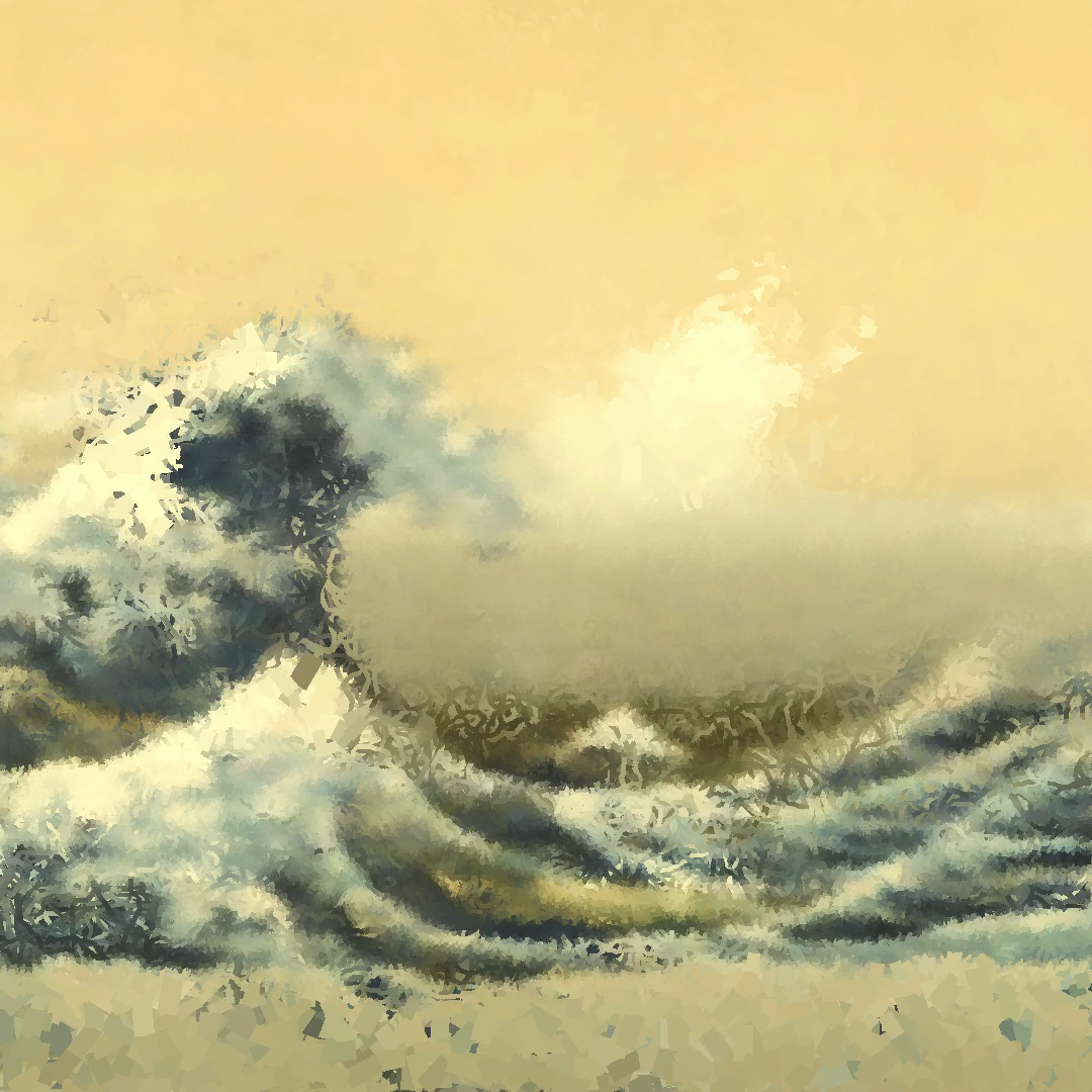
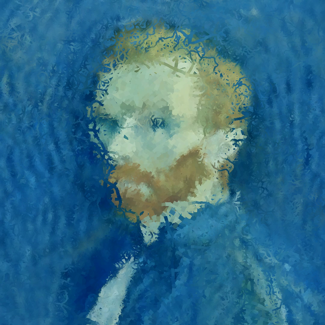
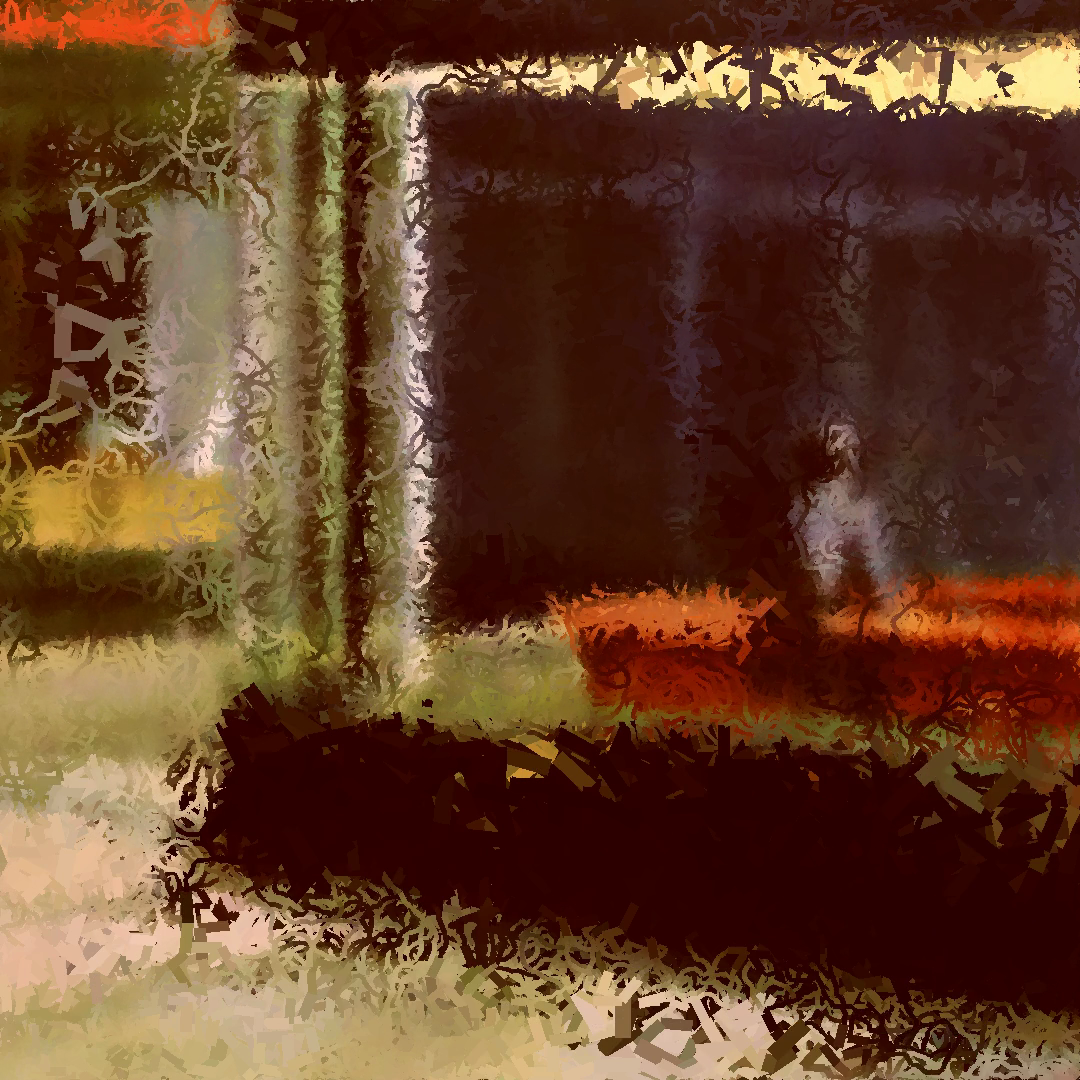
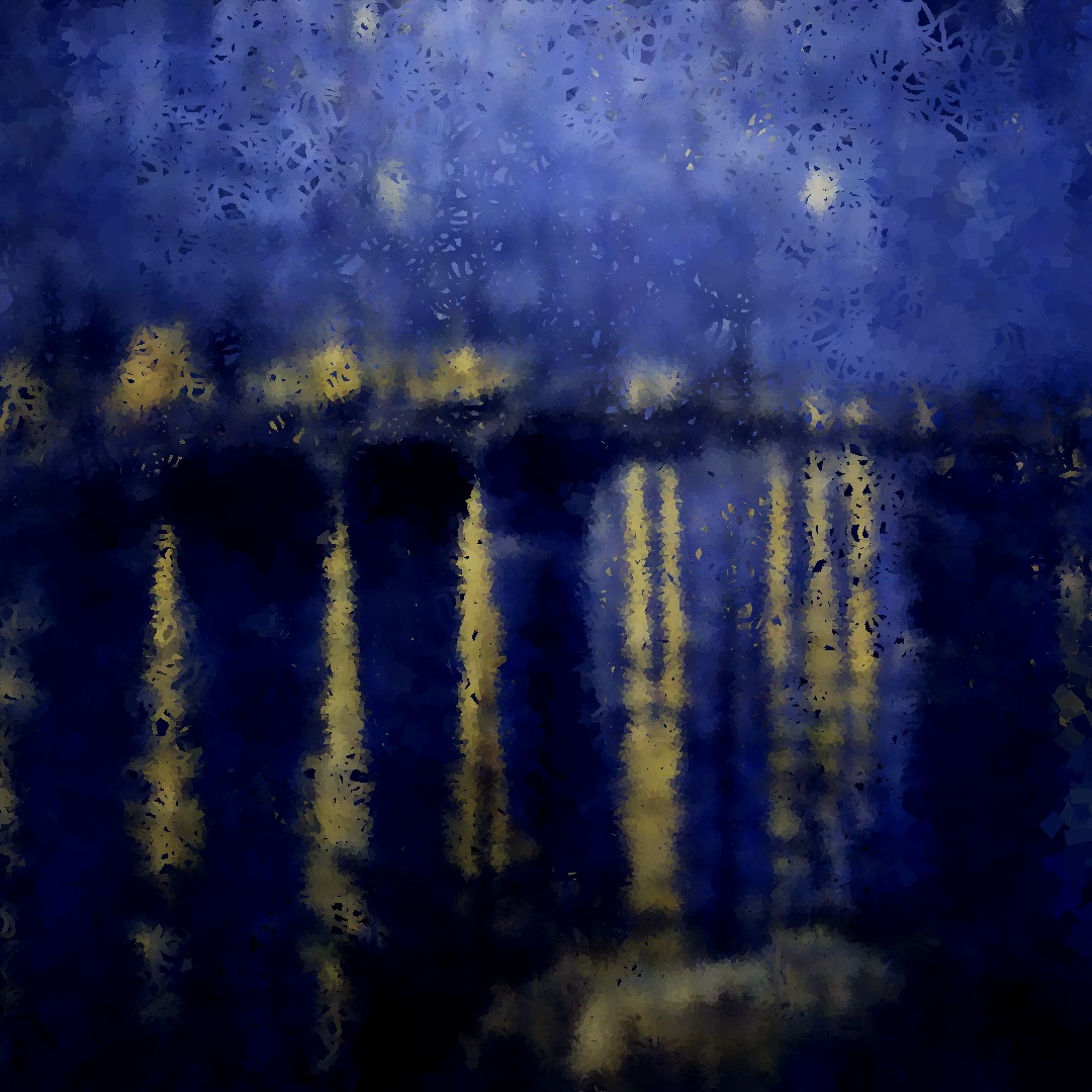
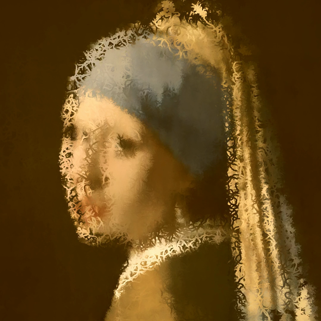
Figure 10. Late frames from five final videos. Each frame is produced by the same workflow, but the reference image, audio features, zoom behavior, and rendering settings lead to different color ranges, stroke textures, and image structures.
How to Read a Result: Do not judge only by the emotional label. Look for visible evidence: color range, readable image structure, stroke density, scale, and how much the canvas has accumulated. These are the signs that connect the result back to the method.
What the Results Show
The results show that the system can turn a still reference image into a moving painting without simply playing the original image as a slideshow. The reference image remains recognizable, but it is rebuilt from many small strokes. This is important because the project is not only about image generation. It is about a painting process that unfolds with music.
The results also show the difference between color learning and painting. The neural network gives the painter a color rule. It helps the system choose colors that belong to the reference image at each location and music frame. The random walk gives the result its visible motion and texture. Because the canvas is not cleared between frames, marks accumulate and the image becomes denser as the video continues.
A single still frame cannot show everything. The final video also contains zoom changes, changes in walker speed, changes in stroke width, and changes in opacity. Those time-based changes are connected to the music features. Therefore, the most complete way to read the output is to compare both a still frame and the moving video: the frame shows the accumulated painting, while the video shows how the painting arrives there.
Summary
Inner Landscapes begins with a simple artistic goal: combine a reference image and a piece of music into a moving painting. To make that goal possible, the project turns both image and music into forms a computer can use.
The music is converted into Mel spectrogram features. A -bin version supplies the current music features for the neural network, and a -bin version helps choose the zoom level. The reference image is prepared at different visual scales so the model can learn how color should change when the selected zoom target changes.
The neural network learns a color rule. Its input is an image location together with the current music features. Its output is a predicted RGB color. During training, the model compares predicted colors with target image colors, uses L1 and L2 loss to measure error, and updates its weights with backpropagation. The checkpoint stores the trained model and the information needed to rebuild the same color rule later.
During rendering, the notebook loads the checkpoint and passes the model to RW_Painter. The painter uses random walkers to create strokes on a larger canvas. The neural network supplies stroke colors, while music intensity and image-region information guide movement, opacity, width, and local drawing behavior. Saved frames are finally combined with the audio to make the final video.
The complete workflow is therefore:
training -> checkpoint -> notebook integration -> RW_Painter rendering -> frames -> final video.
The central lesson of the chapter is that the final artwork is not produced by one technique alone. It comes from the connection between sound features, learned color prediction, visual scale, random-walk motion, and frame-by-frame accumulation.
Appendix
File Map
The main chapter explains the ideas in a teaching order. The program itself is organized by files. The following table gives a compact map for review.
| File | Role in the workflow |
|---|---|
neural_network_music.py | Builds Mel spectrograms, computes zoom levels, defines XYSpecNet, trains the neural color model, saves checkpoints, and contains the video-combining helper. |
random_walk_image.ipynb | Loads a checkpoint, chooses the audio clip and render settings, rebuilds the model, prepares music features for the selected clip, creates RW_Painter, and starts rendering. |
RWraw.py | Defines RW_Painter. This class manages walkers, predicts colors with the trained model, uses image-region information, draws strokes, and saves numbered PNG frames. |
Table 1. Main source files used by the Inner Landscapes workflow.
Core Settings
The following settings are useful when checking whether an explanation, figure, or result matches the implementation.
| Setting | Value or meaning |
|---|---|
| Training image grid | locations |
| Rendering canvas | pixels in the notebook render setup |
| Target frame rate | frames per second for music features and video frames |
| Neural-network music features | Mel values per music frame |
| Zoom-decision spectrogram | Mel values per music frame |
| Fourier coordinate frequencies | Most emotions use ; Nostalgia also uses |
| Model output | Three RGB values between and |
| Final frame format | Numbered PNG files such as 000000.png, 000001.png, and so on |
| Final video step | The saved frames are combined with the selected audio clip |
Table 2. Core settings used throughout the chapter.
Reproduction Checklist
To reproduce the project, follow the same order as the real workflow.
- Prepare the reference image and audio file for each emotion.
- Run the training script so the program can build music features, select zoom targets, train
XYSpecNet, and save a checkpoint. - Confirm that the checkpoint exists before rendering.
- Open the notebook and choose the emotion, audio segment, and render settings.
- Let the notebook load the checkpoint, rebuild the model, normalize the clip’s music features with the saved values, and create
RW_Painter. - Render the numbered PNG frames.
- Combine the frames with the audio clip to create the final video.
Common Problems to Check
| Problem | What to check |
|---|---|
| The notebook skips an emotion | The checkpoint path may be missing. Run the training script for that emotion first. |
| The colors look wrong | Check that the notebook uses the saved spec_min and spec_max from the checkpoint when normalizing the rendering clip. |
| The output does not respond clearly to music | Check that the selected audio segment has enough changing spectrogram energy and that the zoom levels are being sliced for the same time segment. |
| The painting looks too empty early in the video | Remember that the canvas accumulates over time. Early frames naturally contain fewer marks than late frames. |
| The final video is missing audio or does not export | Check that the numbered PNG frames were saved and that the video-combining command can access the audio clip. |
Table 3. Practical checks for reproducing the workflow.