Voronoi Mosaics with Adaptive Sampling and Segment Anything Model (SAM)
Abstract
Using Voronoi Diagrams and Meta’s neural network, the Segment Anything Model (SAM), we can transform any image into a stained glass mosaic by defining boundaries based on an area’s significance due to brightness and edge factors.
Chapter Goals
By the end of this chapter you should:
- Know what a Voronoi Diagram is and why it is so important
- Build a density field for an image using brightness and edge factors
- Create a piece of Voronoi Mosaic art by coding in Python
- Use Meta’s Segment Anything Model (SAM) to generate an object mask
- Combine SAM’s object masks with adaptive sampling to build mosaics that respect object boundaries
Introduction
Look at any photograph for more than a second and you’ll notice something obvious that most image-processing pipelines quietly ignore: not all of it matters equally. A portrait holds its story in the eyes, the corner of a smile, or the tiny lines that make up a dress’ weave; whilst the plain cement wall behind the subject could be summarized in a single stroke and nobody would object. Humans categorize their attention this way instinctively. In this chapter, we’re going to teach a computer to do the same thing, using the technique of Voronoi Diagrams.
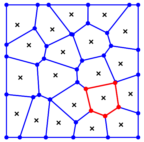 | 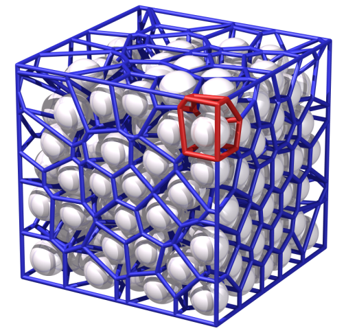 |
|---|---|
| Credit placeholder | Credit placeholder |
The oldest record of the idea comes from René Descartes, sketching out the starry skies by partitioning the space by proximity to the nearest star, in order to map the range of influence of the celestial bodies. Fast forward to 1854, during the cholera outbreak in London, English physician John Snow mapped every home to the nearest water pump in the city, creating a map of “cells,” each with a water pump at its center. Comparing this map with the map of household deaths, he found the vast majority lied in the “cell” of the Broad Street pump. The pump-by-pump territories he sketched were, in effect, Voronoi cells, one of the earliest practical life and death applications of the idea before anyone had named it. In today’s world, this idea has been constantly adapted to fields far beyond epidemiology. In computer science, Voronoi cells power nearest neighbor search and mesh generation, letting a robot or a game engine instantly work out which point between a charging dock, a checkpoint, or a Wi-Fi router it is closest to. In biology, the same geometry describes how cells pack themselves into tissue: each nucleus behaves like a generating point, pushing outward until it collides with its neighbors, which is why a cross-section of skin or plant tissue under a microscope looks uncannily like a Voronoi diagram. And in architecture, the pattern has been used deliberately, the ceiling and façade of Beijing’s National Aquatics Center for the 2008 Olympics, were designed around a Voronoi lattice meant to echo the irregular geometry of soap bubbles. The same math has been used endlessly since centuries ago.
| Title placeholder | Title placeholder | Title placeholder |
|---|---|---|
| [image placeholder] | [image placeholder] | [image placeholder] |
| Name — description — citation | Name — description — citation | Name — description — citation |
The name itself didn’t arrive until 1908, when the mathematician Georgy Voronoi formally generalized the construction to arbitrary dimensions while working on the geometry of quadratic forms, and formalized the definition of Voronoi diagrams as “a partition of space into regions where each region contains all points closest to one generating point, compared with all other generating points.”
In other words, the user chooses a type of scattered point, and categorizes space by which scattered point it is closest to.
Mathematically, let be a metric space with distance function , where . Given a set of sites , we define a cell with as its “seed” or “central point” as
The diagram is simply the collection of for all .
From this historical method of describing star fields and disease prevention, we are going to use it to describe pixels, turning an image into a field of “significance” that lets us decide where we scatter the points in order to create a Voronoi mosaic.
Adaptive Sampling
Methodology
The question we want to answer in this section is “What is important in the image?” We define a pixel’s significance by making a significance field constructed with 2 factors. We look at the brightness, as well as its relationship to surrounding pixels, called the edges. These are defined by the brightness gradient, in other words, how fast the pixel brightness changes as you shift across the image. This allows the detection of an image. In digital image processing, it is called a Sobel filter.
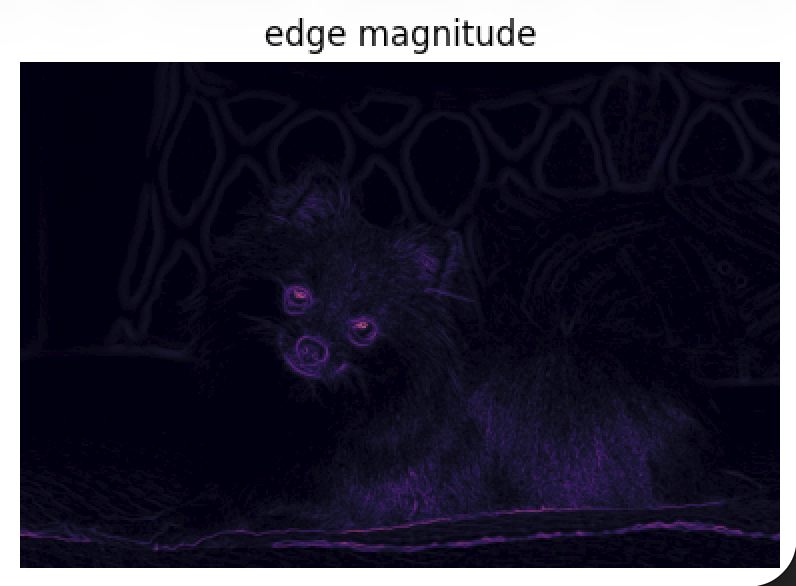
| Original image | 1 − Brightness | Edge magnitude |
|---|---|---|
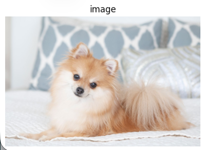 | 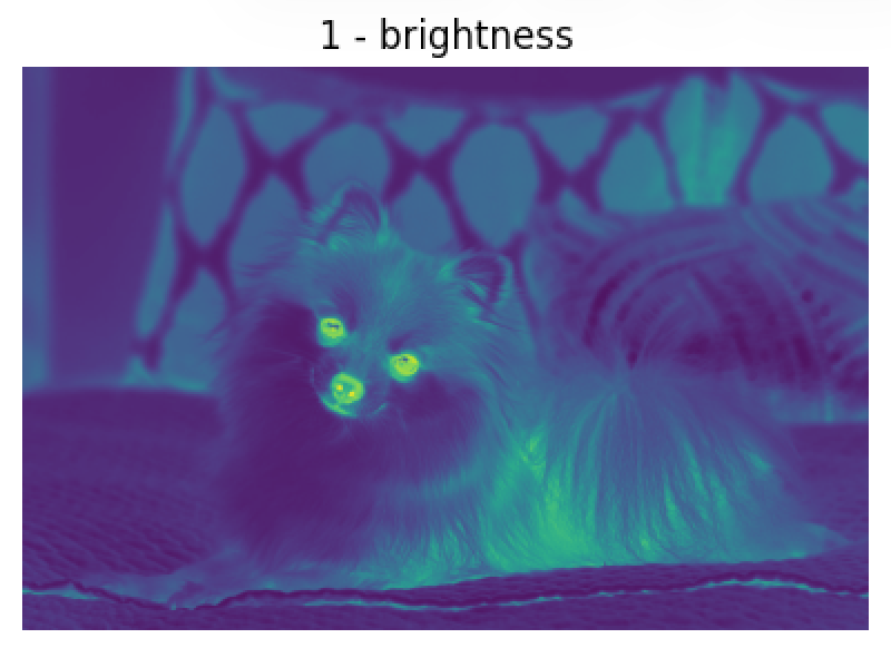 |  |
| Figure 1 — the source image | Figure 2 — the 1 − brightness field | Figure 3 — the edge field |
Figure 2 shows what happens when we look at of the image. We subtract from one because rather than brightness, we are looking for the dark terms. This is because in art, brighter areas are often flattened and lose detail since light erodes nearby detail due to the effect of luminance contrast degradation. In other words, darker areas preserve more details and thus have more “significance.” Figure 3 shows values in which there is a high gradient, such as when we transition from the white fur to pitch black eyes, or the blanket transitions to its shadow.
Overlapping these 2 factors, we get our significance density field, which we can define as . The and terms are so that we can adjust how important we value the brightness factor, or the edge factor. We will get back to this later. For now, we define and , which also happens to align the density field to neatly range from [0,1]. Now, how do we get the brightness and edge terms?
Brightness Filter
Logically, one option to acquire a pixel’s brightness value is to take the red, green, and blue values that range from 0 to 255, and divide them by 3. However, this provides the value for intensity, and not the brightness, due to the fact that human eyes do not perceive red, green, and blue with the same sensitivity. Instead, we can use the standard Rec. 709 colour weights, and define . But why , , and ? Why not just , , and ? The reason is that we must linearize the values. What is linearization? The red, green, and blue values stored in an ordinary image file aren’t physical light measurements. Instead, they are stored as sRGB, a standard method of colour encoding. In sRGB, a nonlinear gamma curve is applied in order to compress brightness values so that darker tones get more precision (which helps with limited 8-bit storage per channel) and also roughly matches how human vision perceives differences in brightness. As such, the RGB numbers in the file do not scale linearly with actual light. For example, doubling a stored value does not mean twice as much physical light. If we were to plug in the sRGB values directly into the Rec. 709 weights, which is what most primitive brightness formulas do, and you get a value called luma: a fast, but not inaccurate approximation of brightness. To get true linear luminance, we first need to undo that gamma curve, converting each channel back to linear light, before weighting and summing them, using these formulas:
and
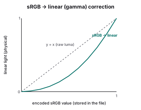
This is the same for green and blue as well. However, we must make sure to normalize our result in the range [0, 1] to work with the linearization process. Thus we now obtain a true brightness formula to compute genuine luminance rather than an approximation.
Sobel Filter
Now that we have discussed brightness, we can discuss how the image’s brightness changes, as a gradient. This allows us to detect edges within an image. Let be the continuous brightness function of the image, then the direction and rate of change of brightness is given by:
However, since in reality is not continuous, but is a discrete function of pixels, we can instead calculate with the slope formula. The gradient terms are then approximated with:
and
which corresponds to convolving the image with the tiny 1-D kernel . The problem is this raw derivative kernel is extremely sensitive to noise. A single stray bright pixel produces a false edge, because nothing in the kernel distinguishes signal from noise. What makes the Sobel Filter more than just a gradient map, and widely used in digital image processing, is because the derivative kernel is combined with a perpendicular smoothing kernel, , which acts as a narrow Gaussian blur that minutely averages neighboring rows. This allows any possible noise to be diluted, not impacting the overall edge detection. Solving for the 2-D Sobel kernel is simply taking the outer product of the x vector and , and y vector with , as such:
With these terms, we can finally define our edge term as:
Image here — A small schematic of the 3×3 Gx and Gy kernels sliding across a patch of pixels to produce a gradient response. It bridges the abstract kernel matrices above and the edge image in the Methodology table, showing what “convolving to find edges” actually does.
Centroidal Voronoi Diagrams & Lloyd Relaxation
In 1957, an engineer at Bell Labs named Stuart Lloyd was wrestling with a problem that, on its face, has nothing to do with images, points, or geometry at all. Telephone engineers wanted to digitize analog voice signals, take any smoothly varying voltage and represent it discretely with finite values. However, too few levels, and the reconstructed voice sounds distorted; too many, and you waste storage. So Lloyd asked, given the distribution of voice amplitudes, quiet sounds are far more common than loud ones, where along the distribution should we place representative levels to make the average reconstruction error as small as possible?
His answer turned out to be a two-step loop that repeated until it stopped changing. First we assign every discrete input value to whichever representative level is closest to it, then we move each representative level to the average of everything just assigned to it, weighted by how often that value actually occurs. That first step, it turns out, is exactly a Voronoi diagram, the preset representative levels act as the central point, whilst every audio input is assigned based on what cell it lands in. The second step is a weighted centroid. Lloyd had rederived the theory of Voronoi diagrams to solve a one-dimensional signal-processing problem. His result circulated informally among engineers for decades before it was formally published in 1982. A near-identical method was found independently by Joel Max in 1960, which is why you’ll sometimes see it called the Lloyd–Max algorithm. It wasn’t until 1999 that mathematicians Qiang Du, Vance Faber, and Max Gunzburger generalized the theory in any number of dimensions, not just one. They thus gave it the name we use today: the Centroidal Voronoi Tessellation, or CVT.
A Voronoi tessellation becomes centroidal when every generating point sits exactly at the center of mass of its own cell. Recall the cell definition from Section 2:
A tessellation built from sites is called centroidal when each satisfies the equation below:
for whatever density we’re weighting by. In Lloyd’s case, it is the probability distribution of voice amplitudes; in ours, the significance field from 3.1. By doing this, we can adjust the scattered points from our density function to sit in their own spaces, “relaxing” them to avoid overcrowding. This matters because in application, a CVT represents a local minimum of a specific quantity, in our case the total quantization error, or distortion represented by:
simply represents how far a typical point sits from its nearest representative, weighted by how much that point matters. A small means our points are doing a good job standing in for the whole density field. What Lloyd’s loop does is coordinate descent on , by holding the partition fixed and moving each to its cell’s centroid can only decrease or leave it unchanged.
| Randomly Scattered Points | 1 Iteration | 10 Iterations | 20 Iterations |
|---|---|---|---|
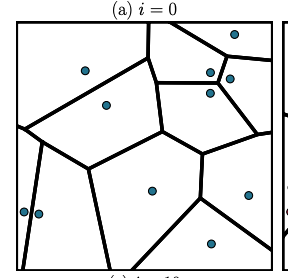 | 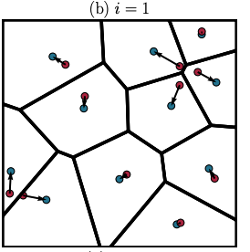 | 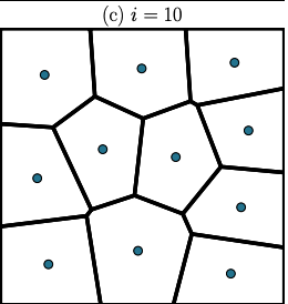 | 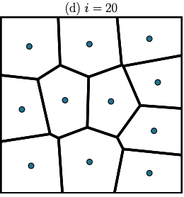 |
| This is the base, a field of randomly scattered points that take up a large range of space. | Upon 1 iteration, the original (red) points move to their new location (blue) which is more central to each cell. | After 10 iterations, the cells become much more uniform as the points reside in their centers. | However after 10 more iterations, not much changes, as we get closer and closer to absolute uniformity. |
Program
Now that we have fully defined our density equation as:
We can create a heat map where we should focus the most amount of points and attention for our Voronoi art as shown in Figure 4. The next step is simply to translate what we have done into Python! Using the Python libraries included in Appendix 1 will allow us to simplify much of the manual mathematics we will have to do, using pre-coded libraries already made.
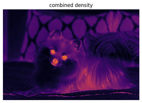
First, we should import our sample image from Appendix 2, and obtain its dimensions in the variables H and W.
url = "https://raw.githubusercontent.com/yue-sun/generative-art/main/02_tuesday/puppy.jpg"
img = np.array(Image.open(BytesIO(requests.get(url).content)))
H, W, _ = img.shape
For the brightness term, we must normalize and linearize as we defined earlier.
def srgb_to_linear(u):
    u = np.clip(u, 0, 1)
    return np.where(u <= 0.04045, u / 12.92, ((u + 0.055) / 1.055) ** 2.4)
This function can now be used to define each linear value.
s = img.astype(np.float32) / 255.0
r_lin = srgb_to_linear(s[..., 0])
g_lin = srgb_to_linear(s[..., 1])
b_lin = srgb_to_linear(s[..., 2])
Now, we can define brightness as:
brightness = 1.0 - (0.2126*r_lin + 0.7152*g_lin + 0.0722*b_lin)
Using the SciPy library, we conveniently can use the sobel function to calculate and without doing the linear algebra ourselves. NumPy simplifies the rest of the other calculations as well.
One thing to note here, the Sobel kernel needs a neighboring pixel on each side to compute a derivative, but the pixels sitting right on the image’s border don’t have a neighbor outside the frame.
Using mode="reflect" handles this by mirroring the image back across its own edge, synthesizing a plausible neighbor instead of assuming black or leaving a gap. Skip it, and you’ll see a false
bright or dark edge framing the entire image. Thus we get:
gx = ndimage.sobel(gray, axis=1, mode="reflect")
gy = ndimage.sobel(gray, axis=0, mode="reflect")
edge = np.hypot(gx, gy)
edge = edge / (edge.max() + 1e-8)
We can then complete significance density function with the line:
density = 0.6*brightness + 0.4*edge
With density fully defined, we’re ready to turn it into actual points. We treat the H × W image as a grid of bins, where each pixel is a bin whose probability of being chosen is proportional to its density
value. Flattening the density field into a 1-D array and normalizing it into a probability distribution lets us draw random pixel indices weighted by density, using rng.choice. We then convert those flat
indices back into (x, y) coordinates, and add a small amount of random jitter to each point so they don’t stack exactly on top of pixel centers as such.
density = np.clip(density, 1e-12, None)
p = density / density.sum()

def sample_points_from_density(p, N, rng):
    h, w = p.shape
    idx = rng.choice(h*w, size=N, replace=True, p=p.ravel())
    ys, xs = np.divmod(idx, w)
    xs = xs + rng.random(N)
    ys = ys + rng.random(N)
    return np.column_stack([xs, ys])

rng = np.random.default_rng(5)
N_points = 8000
pts = sample_points_from_density(p, N_points, rng)
The result is exactly what we planned, a dense cluster of points crowding dark areas, and sparse in the flat images, in other words, the eyes and fur, and a sparse scatter over the flat blanket.
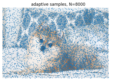
There’s a catch, though. Because sampling is random, points in high density regions can land almost on top of each other, producing small clumps rather than an even mosaic tiling. We fix this with a couple of steps of Lloyd relaxation we discussed earlier, a method to improve spacing without erasing the density pattern. It accomplishes this by iterating many Voronoi diagrams from a set of points, calculating the centroid of each resulting cell, and moving the points into those centers. A cell that’s too small pulls its point outward as it centers itself, and a cell that’s too large does the same in reverse, evening out the spacing without erasing the density pattern that got us here in the first place. However, one or two iterations is enough. Too many iterations will cause the points to drift back toward a uniform grid, removing the chaotic beauty of a mosaic.
The algorithm starts with defining a function finding the center of each cell, by defining the coordinates, and using the shoelace formula for polygon area. We test if the area is close to 0, and if so, it means the point lies on a line, and we simply return an average value. We then implement:
This will thus locate the and values of the centroid.
def polygon_centroid(poly):
    x, y = poly[:,0], poly[:,1]
    A = 0.5*np.sum(x*np.roll(y,-1) - np.roll(x,-1)*y)
    if abs(A) < 1e-10:
        return poly.mean(axis=0)
    cx = np.sum((x+np.roll(x,-1))*(x*np.roll(y,-1)-np.roll(x,-1)*y)) / (6*A)
    cy = np.sum((y+np.roll(y,-1))*(x*np.roll(y,-1)-np.roll(x,-1)*y)) / (6*A)
    return np.array([cx, cy])
As we mentioned before, we need to build the Voronoi mosaic for each iteration, and move the points P to the center of their region to fix/ relax the spacing. We implement with this formula:
def lloyd_box_step(P, W, H):
    V = Voronoi(P)
    out = []
    for r in V.point_region:
        region = V.regions[r]
        if not region or (-1 in region):
            continue
        poly = V.vertices[region]
        if (poly[:,0].min()<0) or (poly[:,0].max()>W) or (poly[:,1].min()<0) or (poly[:,1].max()>H):
            continue
        out.append(polygon_centroid(poly))
    return np.array(out) if len(out) > 50 else P
To iterate it twice, we simply repeat.
relaxed = pts.copy()
for _ in range(2):
    relaxed = lloyd_box_step(relaxed, W, H)
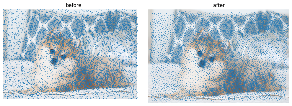
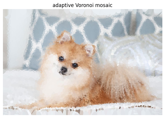
With well spaced points sitting on top of our significance field, the last step is almost anticlimactic: each point becomes the generator of its own Voronoi cell, and we fill that cell with the color sampled from the original image at the generator’s location. Large, flat polygons fall over the smooth blanket; small, tightly packed polygons hug the eyes and the edge of the fur. We can then put everything together like such.
V = Voronoi(relaxed)
fig, ax = plt.subplots(figsize=(7,7))
ax.imshow(img)
for i, r in enumerate(V.point_region):
    region = V.regions[r]
    if not region or (-1 in region):
        continue
    poly = V.vertices[region]
    if poly.size == 0:
        continue
    px = int(np.clip(relaxed[i,0], 0, W-1))
    py = int(np.clip(relaxed[i,1], 0, H-1))
    ax.fill(*zip(*poly), color=(img[py,px]/255.0), linewidth=0)
ax.set_xlim(0,W); ax.set_ylim(H,0); ax.axis('off')
plt.show()
Summary
Starting from a single photograph, we built a significance field out of two humble signals: how dark a pixel is, and how sharply it disagrees with its neighbors. From there, weighted random sampling turned that field into a scatter of points, Lloyd relaxation cleaned up the worst of the clumping without erasing the pattern, and a final Voronoi tessellation turned those points into the mosaic itself. The whole pipeline never once asked what it was looking at, it had no idea it just spent most of its points on a dog’s eyes rather than a blanket, only that the eyes were dark and edgy. That’s both the charm and the limit of adaptive sampling: it’s fast, general, and works on any image you hand it, but it’s blind to meaning. In the next section, we introduce Meta’s Segment Anything Model, which trades some of that generality for genuine object-level understanding, where we tell the algorithm to start becoming specific.
Segment Anything Model (SAM)
Methodology
What we have accomplished so far is create a formula that can take any image, and turn it into a beautiful piece of mosaic art. We successfully created a density function by defining brightness and edge values by first linearizing the image colour values, and even implemented Lloyd’s relaxation algorithm to refine our final art piece. The result is a mosaic that isn’t a random composition of polygons, but one that retains the important nuances of the original using a mathematical idea that has persisted through history. However, what we can do now is create a method that selectively targets only the image subject to become a mosaic. We implement this using Meta’s Segment Anything Model.
Every segmentation model before Meta’s SAM was a specialist. Train it to find cats, and it only finds cats. All the models were unable to generalize. If you wanted to find dogs, you would have to develop a completely new model and train it, and again for birds, and again for anything else. Meta’s Segment Anything project challenged the question, could a single model learn what a boundary is, in general, well enough to segment any object it was never trained to recognize?
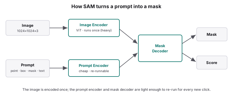
The Segment Anything Model is able to identify anything by going through a few different processes. First it takes a user prompt, which can be text, point, box, or mask. Then the model processes the image through an image encoder using a deep Vision Transformer. Finally, the prompt encoder will find the objects based on the user’s prompt, returning a mask on top of the image identifying the subject. The question though, is how does it know for sure if the item is what the prompt is looking for? The answer is it doesn’t, the given mask is simply the most probable group of pixels to represent the sought object. Internally, the mask decoder doesn’t produce a hard 0 or 1, binary, decision for each pixel at all. Instead it produces a continuous score, and only becomes a binary mask based on a set threshold at the very end. Alongside that mask, the model also reports a confidence score estimating how good its own answer is, similar to, but not exactly a formal probability percentage. The score is a number telling us how much to trust this particular guess. We’ll rely on exactly that score in 4.5, to automatically pick between several candidate masks when a prompt is ambiguous.
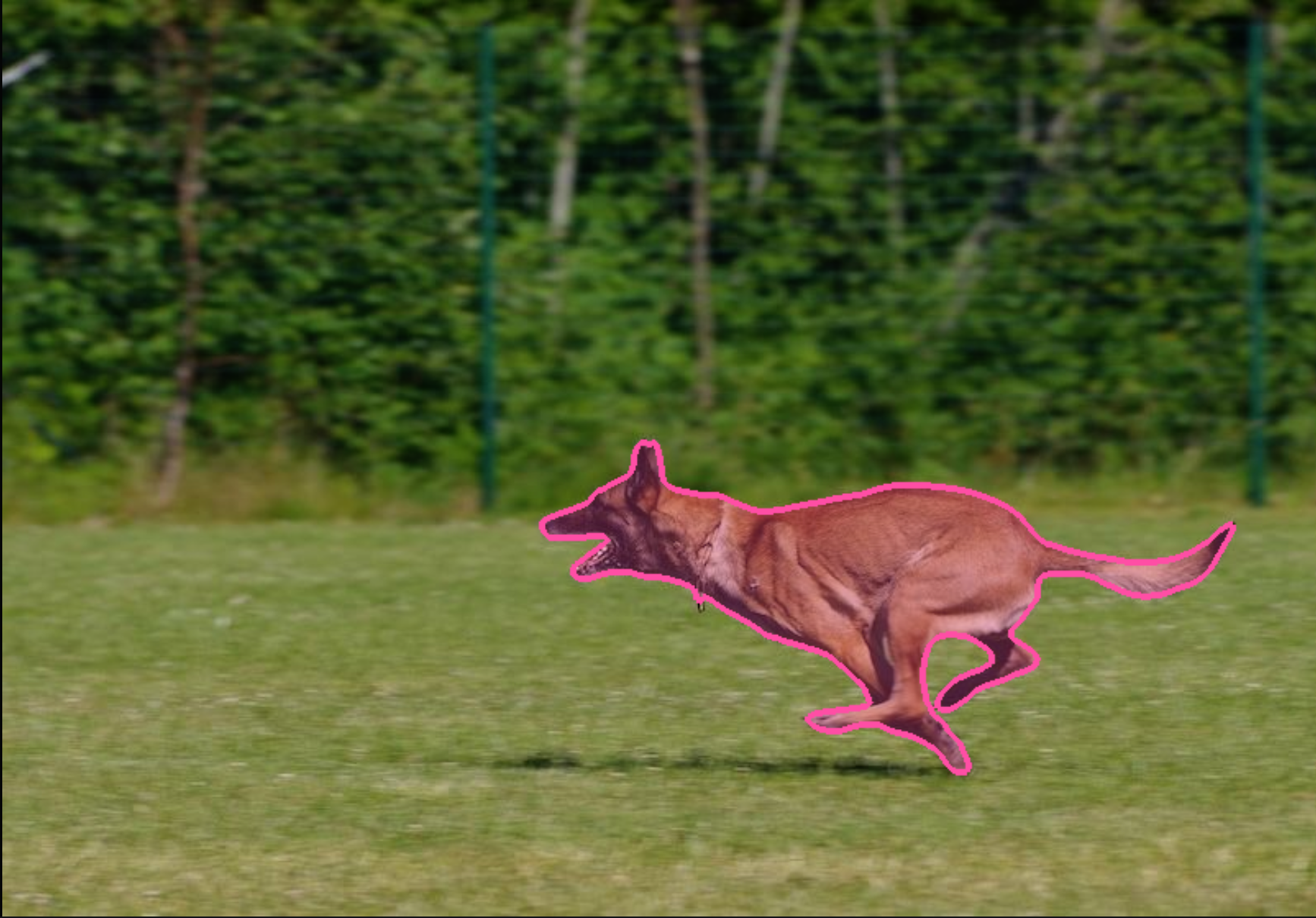
But how does a machine produce that continuous map that scores pixels? Meta’s SAM was trained on 11 million high resolution images, breaking each into about 100 masks per image, totalling a dataset well over 1.1 billion masks. Drawing that many by hand would be near impossible, and so instead most of those masks weren’t drawn by a human at all. With only a small initial round of human-assisted labeling, later stages of the dataset were generated automatically, by earlier versions of SAM itself labeling new images, with humans stepping in only to check quality. This creates a positive feedback loop, where as the model trains itself, it relies less and less on human intervention, and improves at an exponential pace. It’s worth noting for a second, that 1.1 billion masks is roughly a hundred for every single one of the 11 million images, and yet that is still small compared to how many distinct objects exist in the world, which is exactly why zero shot generalization matters so much for a task this open-ended. However, only with that ability to adapt to any task, can we adapt it to this project and selectively “mosaic-fy” any item we wish!
Promptable Segmentation
The first part of the process begins with the prompt. The user inputs what they want to segment, through the process of describing an object with words, a click, or even an automatic mask of everything in the image! But how does a machine understand what the prompt, especially a human sentence, means? In essence, a promptable segmentation model is a function that takes a user image and prompt, feeding it into a function:
This differs from a normal “specialized” segmentation model which only takes in , and identifies on a specific set of pre-trained labels. For a promptable segmentation model, the labels are the user’s prompt, , which allows a user to specify any subject they wish within one model!
Image Encoder
Part 1
The next part of the process is pushing the image through an image encoder. But what is an image encoder? An image encoder is a network that takes in pixels, and understands what each pixel means based on brightness, edges, textures, shapes, or any feature, just like how we detected edges and brightness values for our density function! The image encoder’s job is to turn a 1024×1024×3 image (we resize everything outside of this to that format) into a compact grid of feature vectors, before any prompt has even been considered. This is done only once due to it being a highly computationally expensive task. It’s built from a Vision Transformer, ViT, so the same process language transformers use on words gets applied to pixel clusters. The image is first cut into a grid of fixed 16×16 patches, totalling 4,096, and every patch is flattened and linearly projected into a token. Essentially, each patch is like a word in a language transformer. This is done via a function:
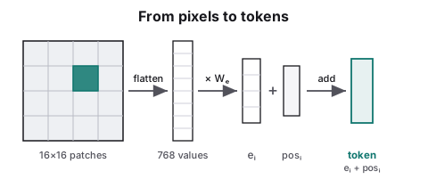
The function simply takes an arbitrary 16×16×3 patch of pixels, , and flattens it. This is simply the process of rewriting the 768 numbers out in one long row instead of a grid, a conversion of information. As for the variable . is a matrix, already found during the extensive training process already done by Meta. This process of training a network is an extensive process in and of itself, but in short, training is done via showing the network millions of images with known correct answers. With every iteration, the model repeatedly adjusts every number inside the matrix in whichever direction pushes it closer to correct. What matters for us is what happens after training finishes: becomes a fixed matrix, baked into the checkpoint file we download. We just don’t know, or need to know, what any individual entry means, just that the matrix has been optimized for the task.
Multiplying these 2 variables gets us , a new vector for every patch. This new vector is called an embedding, and unlike a coordinate vector or color vector such as (x, y) or (R, G, B), none of ‘s individual coordinates have a name. What makes useful isn’t any one number inside it, it’s how relates to the other embeddings. Training pushes visually similar patches toward nearby vectors, and pushes visually different patches apart, regardless of how different their raw pixel values happen to be. To simplify, machines are able to identify similar patches by adjusting the coordinate directions of each embedding, to point towards the same direction, creating a kind of “family” of embeddings.
Now that we understand the patches that compose an image though, we encounter a problem. Nothing in so far records where a patch sits in the image. The function only represents the patch’s own pixels, not the whole’s position. Left alone, a transformer would treat a scrambled ordering of the same 4,096 patches identically to the correct one, since nothing marks which patch is “row 1, column 2”. We fix this with a second vector, , one fixed vector per grid position, also learned during training. We can add this directly onto , and call it a token, carrying both data on what the patch looks like and where it is, represented as:
Part 2
Now we have a job for the transformer. Currently we have 4,096 embeddings, each describing its own patch in isolation. But an image isn’t a bag of independent patches, it must interact with each other to represent a complete image and idea. We want each patch’s embedding to update itself using information pulled from relevant patches. That updating step is called attention, and it’s the core idea underneath every transformer. Every token produces three new vectors from its own embedding, using three more learned weight matrices resulting in:
We can think of as a “query”, what the patch is currently looking for. can be see as a “key”, what the patch has to compare to other patches, and as the “value” of the patch, in other words it is what the -th patch contributes to the whole image.
To decide how much patch should attend to some other patch , we compute the dot product . Using the properties of the dot product, we can tell a lot from the result. The product is large exactly when what patch is looking for lines up with what patch is advertising. For instance, a flower patch’s query vector would tend to align closely with the key vectors of nearby grass patches, and align poorly with a patch of asphalt road. We will also need to divide by purely for numerical stability: and are each vectors of length , so their dot product is a sum of individual terms, and its typical size grows with . By dividing by , we keep these similarity scores in a consistent range regardless of how large happens to be.
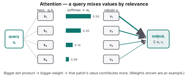
However, these raw similarity scores aren’t weights yet, they can be any real number, positive or negative, and don’t sum to anything in particular. We turn them into a genuine set of weights using the softmax function, which takes a list of scores and returns:
Exponentiating makes every value positive, and dividing by the total makes the whole set sum to exactly 1. As such, the output is a genuine weight map across the whole image, that forces the patch to consider the contributions of every patch, and find out how it relates to them in return.
Finally, patch ‘s updated representation is just a weighted average of everyone’s value vectors, using these attention weights:
Written all at once for every token simultaneously. We stack all the ‘s as rows of a matrix , all the ‘s as rows of , all the ‘s as rows of — this becomes the compact form:
One attention step lets every patch gather information from every other patch, once. SAM’s image encoder repeats this many times, each attention step followed by a small per-token adjustment, and the whole stack is deep enough that information can propagate well beyond just its neighbors.
After all of this, a small final convolution reduces each token’s dimension down to a standard size of 256, and we’re left with:
Which represents a 64×64 grid of 256-dimensional embeddings, one per patch, each one now informed by the entire image, not just its own small corner. Importantly, this entire process of patch cutting, embedding, the many attention iterations, runs exactly once per image before a prompt is taken into consideration.
Prompt Encoder
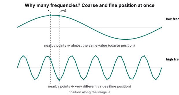
A point prompt starts as a pixel coordinate, an (x, y) vector, but a strange one to handle a network directly. Two nearby coordinates, say (x+1, y) and (x+2, y), differ by a single unit, but their corresponding pixels could call for entirely different masks. If we fed raw coordinates straight into a linear layer the way we fed patch pixels into , the network would have to somehow learn to notice extremely small differences and treat them as possibly meaningful, while also treating some other small differences at a different part of the image as irrelevant. That’s incredibly difficult to train and is inefficient. SAM solves this with a Fourier feature mapping, where instead of feeding (x, y) in directly, it’s first passed through a fixed set of sine and cosine functions at many different frequencies using the function:
where is the coordinate (after rescaling to 1024×1024×3) and is a matrix of frequencies, chosen randomly once and then frozen, never adjusted during training, unlike the weight matrices we’ve seen so far. The intuition is that a low-frequency sine wave changes very gradually across the image, so two nearby coordinates produce nearly identical values under it. This becomes useful for telling roughly which region of the image a point is in. A high-frequency sine wave completes many full cycles across the same image, so it swings rapidly even between very close together coordinates. This makes it much more useful for telling two nearby points apart precisely. Stacking many different frequencies together, from very low to very high, gives the network simultaneous access to both coarse position and fine position, the same coordinate viewed at many different zoom levels at once. This is the same underlying idea as from section 4.3, just built more elaborately, because here it’s not one of several inputs to a token, but the entire content of the token before we add semantic meaning to it.
But only encodes where a point sits, but it says nothing about what kind of point it is. A click meant to say “this is part of the object” and a click meant to say “this is not part of the object” could land at the exact same coordinate and alone couldn’t tell them apart. The fix is the simplest kind of embedding we’ve seen yet. A single fixed vector, we can call it for foreground, for background, and for an unused padding slot. This is enforced for the machine to memorize once during training, with no individual coordinate we could point to and explain, just like the embedding vector. Whichever one applies gets added directly onto the positional encoding:
As such the final token knows both where a point is, as well as what kind of “thing” that point is as well.
A box prompt just reuses this twice. The two opposing corners of a box are each encoded exactly like a point: and . Each gets its own label vector, top left, , or bottom right, , marking which corner it is. Thus we have for box prompts:
Rather than building a separate encoder for an entirely different prompt shape, SAM just teaches two more tokens, what “top-left corner” and “bottom-right corner” mean, and reuses the same pipeline.
Image here — A simple schematic of the prompt types: a foreground click vs a background click at the same spot, and a box drawn as two labelled corners. It shows how each different prompt shape turns into a token, tying together the label vectors and the box encoding just described.
Mask Decoder, Ambiguity, and Multi-Mask Output
By now we have built two separate pieces, the function , the 64×64 grid of patch embeddings from the 4.3, and the prompt token we built in 4.4 that locates our target. In order to put the puzzle pieces together however, we use a Mask Decoder that allows these to talk to each other, using the attention formula we already derived:
It does this in a fixed three step order, repeated twice. First, the prompt tokens attend to each other, i.e. self-attention, exactly as in 4.3, just among the handful of prompt tokens (or often a single token) rather than the 4,096 image patches. This lets a background point cancel out a nearby foreground point’s influence before either one even looks at the image. Second, the prompt tokens attend into the image embedding, cross attention, where the query vectors now come from the prompt tokens but the keys and values come from the function , pulling in whatever visual detail is relevant to what was clicked. Third, the image tokens attend back out to the prompt tokens, letting the whole image representation absorb what the prompt was asking for. Run this three step exchange twice, and the decoder is done talking to itself.
Image here — A diagram of the decoder’s two-way attention: the prompt and output tokens and the image grid exchanging information (tokens → image, then image → tokens), repeated twice. Seeing the back-and-forth makes the abstract “talking to each other” step concrete.
Mixed in among the prompt tokens for this entire exchange are a handful of extra tokens that don’t represent any point or box at all, we call them “output tokens”. They start as generic, freshly initialized vectors, and their only role is to sit through the same attention process as everything else, quietly absorbing information about the image and the prompt as they go. By the end, each output token holds a compressed description of the best candidate answer. The concluding step, comparing that token against every one of the other 4,096 image tokens, expands it back out into an actual pixel by pixel mask.
There’s still a problem originating from our prompt though, causing ambiguity in our answer. When you use a point prompt, the same point can refer to a multitude of items. Clicking on a car tire could refer to the car, the tire, the treads, or the bolts on the side. Instead of forcing one output token to somehow encode a single “correct” answer, SAM uses three of them, plus a fourth dedicated purely to scoring. Each of the three tokens are pre-trained, and specialize towards different scales, for sub parts, a part, or the whole object. Because of how they’re trained, for any given training example, only the best-matching of the three candidates gets reinforced, never all three averaged against the same target. That’s what lets the three specialize into genuinely different answers instead of collapsing into three copies of the same blurry compromise due to averaging. The fourth token’s job is separate and simpler: predict numerically, how good each of the three candidate masks are. It acts as an estimate trained against the real overlap score, and exactly the number the code calls the “score”.
Table here — A three-column comparison of the candidate masks for one ambiguous click (sub-part, part, and whole object), each shown with its predicted score. It makes “multi-mask output” and the scoring token tangible, and shows why the highest-scoring mask is the one we keep.
Refining
Refinement isn’t really a new mechanism added on to the model, but just the same mask decoder from 4.5 but ran another time, with two small changes. The first change is easy, a second point handled exactly like the first, just one more token added to the prompt.
The second change is a bit more nuanced. Beyond points, boxes, and text, SAM supports a fourth kind of prompt: a dense mask. A full-resolution rough sketch, meant for a person to draw as a hint about roughly where the object is. Refinement reuses this exact process, except the “rough sketch” isn’t drawn by a person, but the model’s own previous output. Recall from 4.5 that before thresholding into a hard mask, the decoder’s raw output is a continuous, pixel by pixel score called logits: not yet a yes or no answer, but a field that still carries the model’s uncertainty. The field is high where it’s confident an object is present, low where it’s confident it isn’t. Feeding that back in as a mask-type prompt is mechanically no different from a person sketching a rough hint by hand, shown in the function:
where shrinks last round’s heat map down and mixes it directly into the image embedding . It doesn’t get turned into a token sitting alongside the points, but blended into the image side itself, the same way got blended into a patch embedding back in 4.3. By the time round runs, already carries a rough memory of where the object was. The new point in just needs to nudge that memory, not rebuild it from a blank page. Add a foreground point to claim territory the model was too conservative about, or a background point to carve out something it was too generous with, and the correction only has to account for what changed.
With this understanding of the backend, we can build up our mask encoder and apply our Voronoi Mosaic selectively.
Image here — A before-and-after of refinement: the mask from a single click, then the improved mask after adding a second point and feeding the previous logits back in as a warm start. It makes the warm-start idea visible — the correction only has to fix what changed, not rebuild the mask from scratch.
Program
As with adaptive sampling, we need a few libraries before starting. This time we can include Meta’s own segment-anything package and a pretrained checkpoint, which is a few gigabytes, so expect the download to take a moment.
!pip -q install opencv-python
!pip -q install 'git+https://github.com/facebookresearch/segment-anything.git'
!wget -q -O truck.jpg https://raw.githubusercontent.com/facebookresearch/segment-anything/main/notebooks/images/truck.jpg
!wget -q -O sam_vit_h.pth https://dl.fbaipublicfiles.com/segment_anything/sam_vit_h_4b8939.pth
SAM’s own demo image is more useful here than another shot of the puppy, a truck gives us hard edges, flat panels, and a clean background, which makes it easier to see exactly what a point prompt does and doesn’t capture. One step to note however, OpenCV loads images in BGR channel order, not RGB, so we need to flip that before doing anything else.
import cv2

image_bgr = cv2.imread("truck.jpg")
image = cv2.cvtColor(image_bgr, cv2.COLOR_BGR2RGB)
H, W = image.shape[:2]
A point prompt is just a pixel coordinate and a label. “1” stands for “this is part of the object,” “0” stands for “this is explicitly not.” We’ll start with a single foreground point, dropped roughly in the middle of the truck’s cab.
input_point = np.array([[500, 375]])
input_label = np.array([1])
Now for the two call split from 4.3. Loading the model and calling set_image runs the computationally heavy image encoder exactly once.
import torch
from segment_anything import sam_model_registry, SamPredictor

sam = sam_model_registry["vit_h"](checkpoint="sam_vit_h.pth")
sam.to(device="cuda" if torch.cuda.is_available() else "cpu")
predictor = SamPredictor(sam)
predictor.set_image(image)
With the image embedded, a single call to predict() runs the cheap half of the network, the prompt encoder and mask decoder from 4.4 and 4.5. Remember that an ambiguous prompt gets three candidate masks back, so we ask for all three and keep the
one with the highest score.
masks, scores, logits = predictor.predict(
    point_coords=input_point,
    point_labels=input_label,
    multimask_output=True,
)

best_idx = int(np.argmax(scores))
best_mask = masks[best_idx].astype(bool)
Image here — The three candidate masks SAM returns for the single cab click, side by side with their confidence scores and the best one highlighted. It shows the ambiguity problem and the score-based selection playing out on the real truck image. (Generated by running the notebook above.)
One point on a truck’s cab is ambiguous in exactly the way 4.2 and 4.5 described. If the best mask stops short of the full truck, we refine rather than restart, exactly as in 4.6: pass the previous logits back in as a warm start, and add a second foreground point further along the truck bed.
refined_points = np.array([[500, 375], [1125, 625]])
refined_labels = np.array([1, 1])

refined_masks, _, _ = predictor.predict(
    point_coords=refined_points,
    point_labels=refined_labels,
    mask_input=logits[best_idx][None, :, :],
    multimask_output=False,
)

final_mask = refined_masks[0].astype(bool)
Image here — The refined mask overlaid on the truck after the second point and the logits warm-start. Placing it next to the previous result shows how one extra click completes the object. (Generated by running the notebook above.)
From mask to mosaic. With final_mask in hand, everything from Section 3 becomes available again, just restricted to a shape instead of a rectangle. srgb_to_linear, r_lin/g_lin/b_lin, and the Sobel gradient from 3.5 all carry over unchanged.
The only new line is the one that matters, multiplying the density field by the mask, so every pixel outside the truck drops to zero density and can never be sampled.
luminance = 0.2126*r_lin + 0.7152*g_lin + 0.0722*b_lin

edge = np.hypot(ndimage.sobel(luminance, axis=1, mode="reflect"),
                ndimage.sobel(luminance, axis=0, mode="reflect"))
edge = edge / (edge.max() + 1e-8)

density = 0.6*(1.0 - luminance) + 0.4*edge
density = density * final_mask.astype(np.float32)
Sampling is exactly sample_points_from_density from 3.5, a pixel with zero density simply never gets picked, so masking comes “for free.”
density = np.clip(density, 1e-12, None)
p = density / density.sum()

rng = np.random.default_rng(123)
pts = sample_points_from_density(p, N=4000, rng=rng)
Relaxation is the same story, almost. lloyd_box_step from 3.5 still works unchanged, it just moves each point to the geometric centroid of its own Voronoi cell within the image’s bounding box. But “within the bounding box” is exactly the problem
here: a centroid can legally sit inside that rectangle while sitting outside our curved mask, in the empty space beside the truck. Left alone, a few points drift there every iteration and never come back.
The fix is a nearest-inside-pixel lookup, computed once with a distance transform: for every pixel outside the mask, it tells us the coordinates of the closest pixel that’s inside.
dist, (iy, ix) = ndimage.distance_transform_edt(~final_mask, return_indices=True)

def project_to_mask(points, mask, ix, iy):
    x = np.clip(points[:,0].astype(int), 0, mask.shape[1]-1)
    y = np.clip(points[:,1].astype(int), 0, mask.shape[0]-1)
    outside = ~mask[y, x]
    points[outside, 0] = ix[y[outside], x[outside]]
    points[outside, 1] = iy[y[outside], x[outside]]
    return points
Run one relaxation step, then snap anything that escaped back inside, and repeat:
relaxed = pts.copy()
for _ in range(2):
    relaxed = lloyd_box_step(relaxed, W, H)
    relaxed = project_to_mask(relaxed, final_mask, ix, iy)
The last step needs its own idea, not just a reused one. Filling explicit Voronoi polygons, like we did back in 3.5, means clipping each cell against a boundary. The thing is, clipping against a rectangle, the image edge, is easy, but clipping against an arbitrary curved mask boundary can be a real challenge geometrically that won’t be solved by an if statement.
So instead of building polygons at all, go back to the actual definition of a Voronoi cell from Section 2: the set of points closer to one generator than to any other. That’s a rule about individual points, not about polygons, nothing requires us to express it as a shape. We can ask the question one pixel at a time, for every pixel inside the mask, which of our relaxed points is nearest? We answer that with a spatial lookup structure, a k-d tree makes this fast even for a few thousand points, and the result is, by definition, the correct Voronoi partition, automatically clipped to the mask, because we only ever asked the question for pixels already inside it.
from scipy.spatial import cKDTree

ys, xs = np.where(final_mask)
mask_pixels = np.column_stack([xs, ys])

tree = cKDTree(relaxed)
_, nearest = tree.query(mask_pixels)
Each pixel now knows which generator it belongs to. Coloring the mosaic is one more lookup: take the color the original image had at each generator’s own location, and hand it to every pixel assigned to that generator.
gen_colors = image[relaxed[:,1].astype(int), relaxed[:,0].astype(int)]

mosaic = image.copy()
mosaic[ys, xs] = gen_colors[nearest]

plt.figure(figsize=(8,8))
plt.imshow(mosaic)
plt.axis("off")
plt.show()
Image here — The final masked Voronoi mosaic of the truck. It’s the payoff of the whole section — detail only where SAM told us to look — and sits naturally beside the dog mosaic from Adaptive Sampling for a direct comparison. (Generated by running the notebook above.)
The truck comes out tiled in exactly the same spirit as the puppy did, dense where the density field says there’s detail, sparse where it doesn’t. However, now that detail only exists where SAM told us to look. Section 3 taught the algorithm where to place points; Section 4 gave us a system on where to stop.