Abstract
Chapter 4 developed a neural color rule. This chapter turns that rule into a moving painting. Random walkers leave colored strokes on an accumulating canvas. Current music intensity affects movement and stroke appearance, and image-region information varies local drawing behavior. The rendering notebook connects a trained checkpoint to the painter, then combines numbered frames with the selected audio clip.
Chapter Goals
-
Describe walker position, direction, and random turning.
-
Explain the effects of music on motion, width, and opacity.
-
Understand local emotion-style and detail-style controls.
-
Follow notebook integration, frame rendering, and video export.
Introduction
A predicted color does not determine the route of a brush. A random walk creates that route through many small steps, allowing the direction to change at each step. Many walkers can build a painting across the canvas at the same time.
A simpler music-painting approach can use a hand-designed mapping from audio features to color. Neural guidance replaces that mapping with the learned image representation from Chapter 4. The walkers still create the path; the network supplies color from image location and current music features.
This chapter explains the painting method and program. Chapter 11 develops the creative intent behind the resulting five-work series.
Methodology
Overall Methodology
The question we need to answer is: how do we turn a still reference image and a changing piece of music into a painting that changes over time? At the conceptual level, the workflow is:
reference image + music music representation and zoom targets train neural network random-walk painting saved frames final video.
Chapter 4 develops the training stage: a reference image and music provide examples on a grid, with three zoom targets representing different visual scales. The resulting checkpoint stores the learned color rule and the settings needed to restore it, including spectrogram normalization, music frame rate, and zoom information. This checkpoint is the bridge to the rendering stage studied here.
The second part of the pipeline happens during rendering. The notebook chooses an audio segment, rebuilds the music features for that segment, loads the trained neural network from the checkpoint, and creates a random-walk painter. The painter starts with a blank canvas. At each frame, each walker takes many small steps. At each walker location, the neural network uses the current image location and current music features to predict the stroke color. The music also affects the walker movement and stroke appearance. Image-region information derived from the reference image lets different parts of the canvas behave differently.
The canvas is saved many times as a sequence of still images, called frames. These frames are then combined with the music to create the final video.
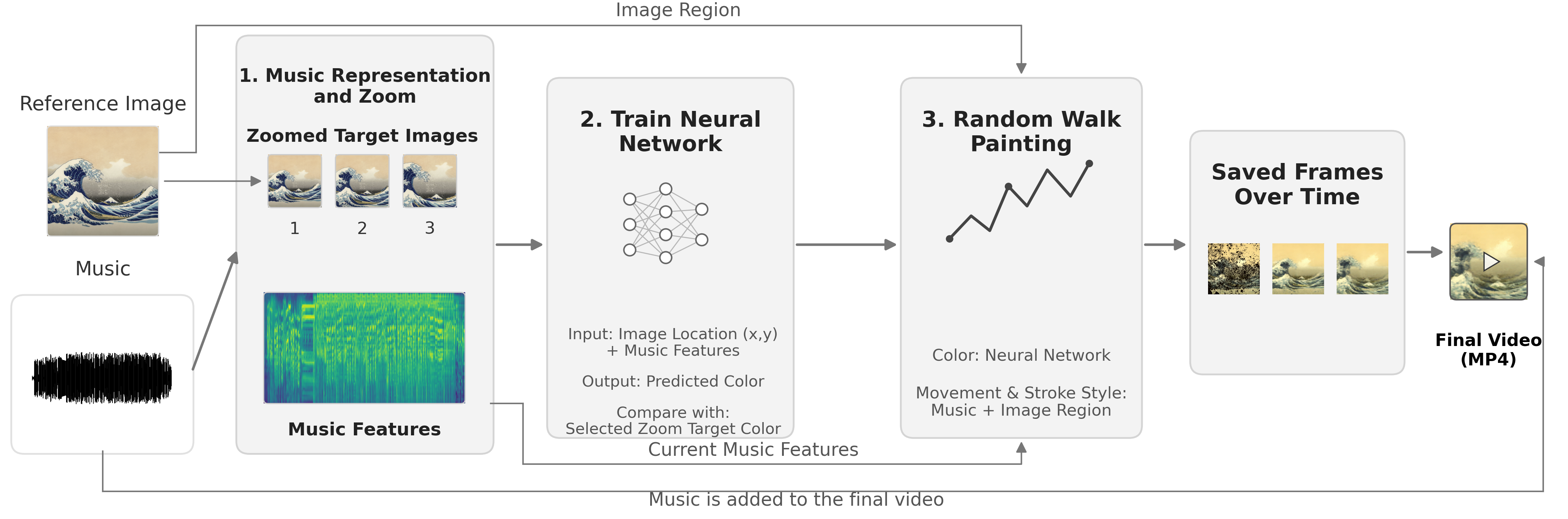
Figure 5.1 gives us a simple map of the process. Chapter 4 develops the music representation and neural training in this workflow. Here we continue from the checkpoint to painting and video.
Audio-Driven Random Walk Painting
From Color Rule to Moving Strokes
The neural network can predict colors, but it does not decide where to draw. The moving painting needs a path. In Inner Landscapes, that path is created by random walkers.
A random walker has a current position and a current direction. We can write its state at step as
where is the walker’s position and is the direction angle. At each small step, the direction changes by a random amount. In the code, this random turn is sampled from a normal distribution:
so the new direction is approximately
The walker then moves forward using basic trigonometry:
where is the step length. This is the essential mathematics of the random walk used here: turn a little, move forward, repeat. If the next position reaches the boundary of the canvas, the direction is reflected back into the image. This keeps the walker inside the painting area. The walkers do not begin from one single point. They are initialized across a grid of canvas cells, so the painting can start building in many regions.
The notebook does not train the model again. It loads the checkpoint, rebuilds the neural network, restores the saved weights, cuts the chosen audio segment, and recomputes the music features for that segment using the same normalization values saved during training. Then it creates an RW_Painter.
At frame , the painter takes the current music features . The model uses these features for color prediction. The painter also computes a simple music intensity value:
This intensity value controls how active the walkers become. A stronger frame produces longer steps, thicker strokes, larger turning variation, and higher opacity. In simplified form, the base controls are
Emotion-specific parameters then scale these quantities. For example, a piece can use more walkers, larger step scale, stronger turning scale, or a different color tint. These choices affect the visual style of the piece without changing the basic rule: music features and image location still determine the predicted color.
Key Distinction: Music features have two jobs during rendering. The full current music vector is used by the neural network to predict color. The single intensity value from that vector is used by the painter to control motion and stroke appearance.
Image-Region Information and Local Style
The painter also uses image-region information from the reference image. This information does not replace the neural network. It affects how the walkers move and how strongly they draw in different parts of the canvas.
The program first converts the reference image to grayscale and measures edge strength with image gradients. Then it selects lower-edge regions, blurs that selection, and turns the result into a region weight between and . During rendering, the active region map is matched to the current zoom level, so the region guidance follows the same visual scale as the selected zoom target.
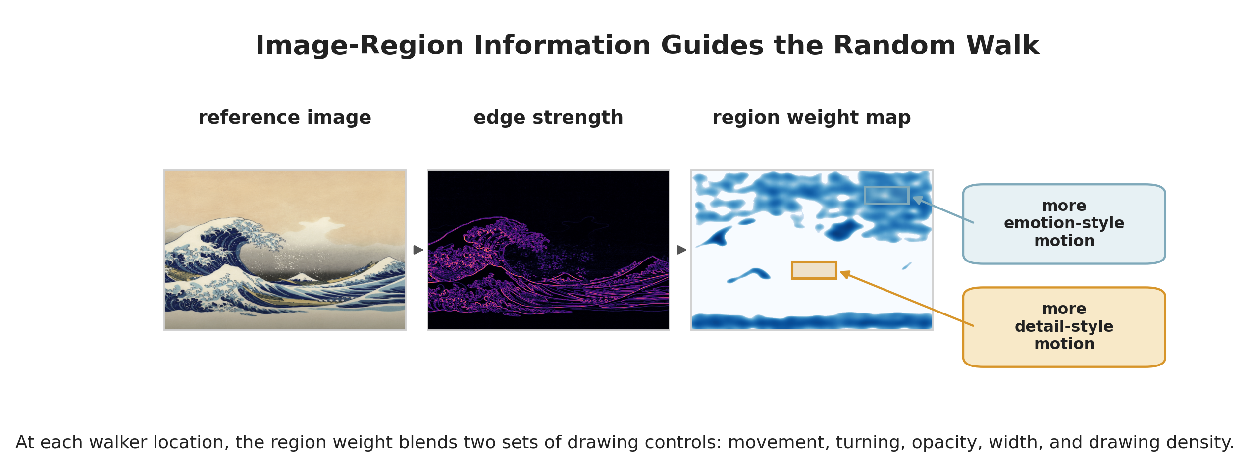
Figure 5.2 shows why the region map is useful. Some locations use more emotion-style behavior, which can mean stronger movement, opacity, width, or drawing density. Other locations use more detail-style behavior, which is usually softer and more controlled. The final stroke parameters are blended from these two behaviors at the walker’s current location.
The blend is a simple weighted average. If is the region weight at the current walker location, then a local control value can be written as
Here can stand for step length, turn variation, opacity, stroke width, or the number of drawing steps used in one frame. When is close to , the emotion-style control dominates. When it is close to , the detail-style control dominates. Values between and smoothly mix the two.
Each walker step follows the same basic sequence:
choose local drawing controls turn move predict color draw a stroke.
The canvas is not cleared between frames. Each new stroke is added on top of the previous strokes. This is why the result feels like a painting being built over time rather than a set of unrelated images.
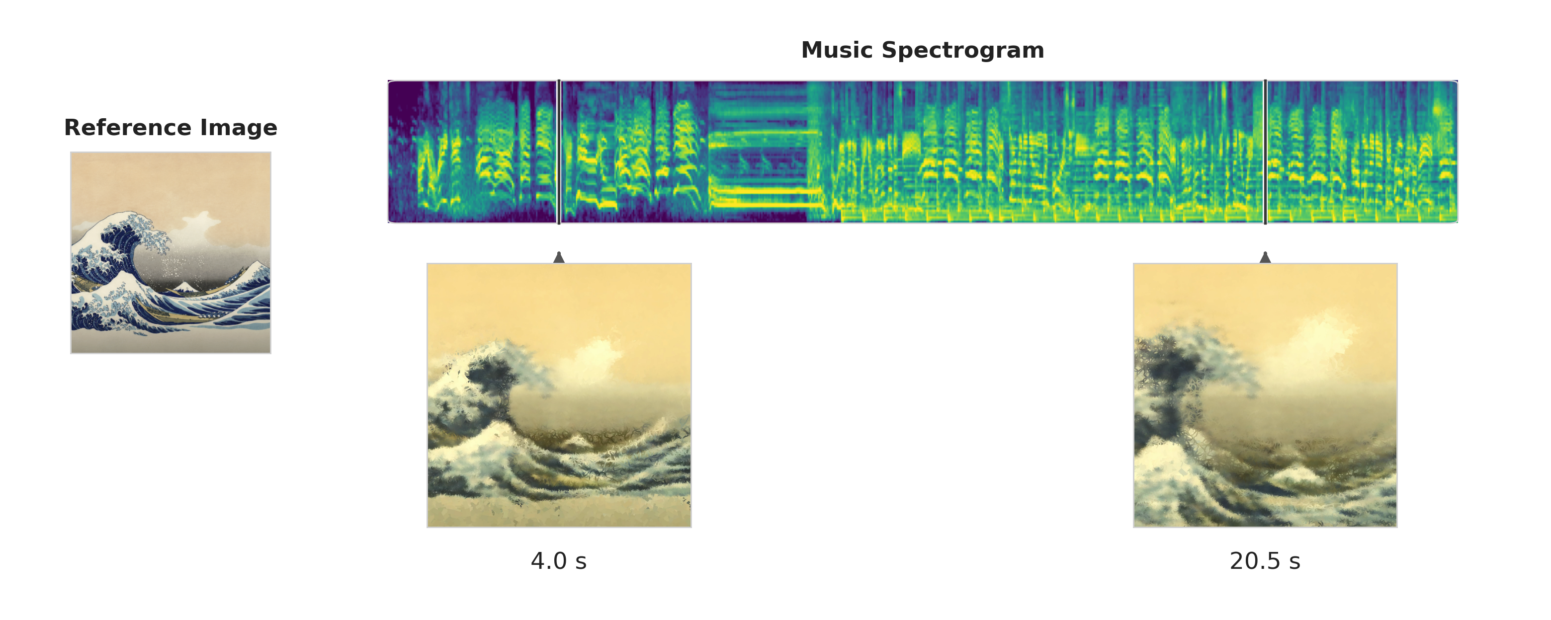
Figure 5.3 shows this time-based behavior. The reference image gives the visual world, the spectrogram gives changing music features, and the random walkers turn those features into accumulated marks. After the painter saves all frames, the frames are combined with the audio to create the final video.
Program
The Methodology section explained the ideas. This section connects those ideas to the actual program. The goal is not to memorize every line of code. The goal is to know where each part of the system happens and how data moves from one file to the next.
The code is organized around three main files:
| File | Main job |
|---|---|
neural_network_music.py | train the neural color model and save checkpoints |
random_walk_image.ipynb | load checkpoints, choose audio clips, and start rendering |
RWraw.py | run the random-walk painter and save frames |
As in Chapter 4, the code blocks below are excerpts from the complete source files. They show how information moves through the program rather than replacing its full setup.
The real implementation follows the engineering workflow introduced earlier:
training checkpoint notebook integration RW_Painter rendering frames final video.
This is the code-level version of the conceptual workflow. The conceptual workflow tells us what the system means. The code workflow tells us where the files hand information to one another.
Notebook Integration
Rendering begins in random_walk_image.ipynb. The notebook imports the trained model class and helper functions from neural_network_music.py, and it imports the painter from RWraw.py:
from neural_network_music import XYSpecNet, make_mel_spec, normalize_spec
from neural_network_music import frames_to_video_with_audio
from RWraw import RW_Painter
The notebook then loads one checkpoint:
ckpt = torch.load(ckpt_file, map_location="cpu")
latent_size = ckpt["latent_size"]
hidden = ckpt["hidden"]
target_fps = ckpt["target_fps"]
These values tell the notebook how to rebuild the network. The model must have the same input dimension, hidden size, and Fourier encoding that were used during training.
The notebook rebuilds the neural network and restores its learned weights:
model = XYSpecNet(
    spec_dim=input_spec_dim,
    hidden=hidden,
    fourier_frequencies=model_fourier_frequencies,
)
model.load_state_dict(ckpt["model_state_dict"])
model.eval()
The call to model.eval() puts the model in evaluation mode. In simple terms, the model is no longer learning. It is now being used to make predictions.
The notebook also cuts the selected audio segment and recomputes the music features for that segment:
make_audio_clip(audio_file, start_sec, end_sec, clip_file)
raw_spec = make_mel_spec(clip_file, latent_size, target_fps)
spec, _, _ = normalize_spec(raw_spec, spec_min=spec_min, spec_max=spec_max)
Notice that the same spec_min and spec_max from training are reused. This keeps the meaning of the music-feature values consistent between training and rendering.
The notebook also slices the saved zoom levels so that the zoom behavior lines up with the chosen audio clip:
zoom_start_frame = int(round(start_sec * target_fps))
zoom_levels = full_zoom_levels[
    zoom_start_frame:zoom_start_frame + num_frames
]
This step matters because rendering may use only part of the original audio file. The zoom levels must start at the same musical time as the clip.
RW Painter Rendering
The notebook creates an RW_Painter. This object owns the canvas, the walker positions, the walker directions, the image-region map, and the drawing process:
painter = RW_Painter(
    model, W_RENDER, H_RENDER,
    num_walkers=cfg["num_walkers"],
    emotion_params=emotion_params,
)
The model gives the painter a way to predict color. The render size gives the painter the canvas size. The walker count and emotion parameters control how many walkers move and how their strokes behave.
Then the notebook starts rendering:
painter.render(
    spec=spec,
    num_frames=num_frames,
    steps_per_frame=cfg["steps_per_frame"],
    output_dir=output_dir,
    target_fps=target_fps,
    zoom_levels=zoom_levels,
)
Inside RWraw.py, the render method loops over the frames. For each frame, it selects the current music features, chooses the active zoom-level region map, computes music intensity, updates every walker, predicts stroke colors with the neural network, and draws lines onto the accumulating canvas.
Each saved frame is named with six digits:
frame_path = os.path.join(output_dir, f"{f:06d}.png")
self.canvas.save(frame_path)
This naming pattern is important because video tools expect frames to be in a clean numerical sequence, such as 000000.png, 000001.png, and 000002.png.
Frames and Final Video
The last step is handled by frames_to_video_with_audio. The notebook calls it after all frames have been rendered:
frames_to_video_with_audio(
    output_dir=output_dir,
    output_name=output_name,
    audio_file=clip_file,
    target_fps=target_fps,
)
This helper function uses ffmpeg twice. First, it turns the numbered PNG frames into an MP4 video. Then it adds the audio clip to that video. The final result is a video file whose images and audio share the same frame rate and duration.
Useful Rule: In the code, training and rendering are separate.
neural_network_music.pylearns and saves the color rule.random_walk_image.ipynbreloads that rule.RWraw.pyturns the reloaded rule into painted frames.
Exercises
These questions connect the painting process to the learned representation in Chapter 4.
Zoom and Random-Walk Rendering
-
A random walker has state . What does each part of this state represent?
-
If a walker starts at , has direction , and takes a step of length , what is its new position before any boundary reflection?
-
If the current music intensity increases, what happens to step length, stroke width, turn variation, and opacity?
-
A local drawing control is computed as . If , , and , compute .
-
Why is the canvas not cleared between frames?
Program Workflow
-
Put these stages in the correct order: notebook integration, final video, training,
RW_Painterrendering, checkpoint, frames. -
Which source file defines
XYSpecNet? -
Which source file defines
RW_Painter? -
Which file loads the checkpoint and starts the rendering process?
-
If an audio clip lasts seconds and the target frame rate is frames per second, about how many frames should be rendered?
-
Why does the notebook reuse
spec_minandspec_maxfrom the checkpoint when it normalizes the rendering audio clip? -
What does
frames_to_video_with_audiodo after all PNG frames have been saved?
Results
The final output of the project is a video, but a still frame is a useful way to study what the system has produced. A finished frame shows the accumulated canvas after many random-walk strokes have already been drawn. By this point, the frame contains information from the reference image, the trained neural color rule, the selected zoom targets, and the changing music features.
Figure 5.4 shows one late frame from each final video. These frames should not be read as five isolated pictures. They are snapshots from moving paintings. The visible result at any moment depends on what the music has done up to that time and how the canvas has accumulated previous strokes.
How to Read the Output
When looking at the results, it helps to ask three concrete questions.
First, what color world does the frame use? The Joy frame is dominated by pale yellows, greens, and blue-gray wave shadows. The Calm frame uses mostly cool blues and soft green highlights. The Anxiety frame contains stronger dark reds, browns, and high-contrast light areas. The Grief frame is mostly deep blue with vertical yellow reflections. The Nostalgia frame uses warm browns, golds, and muted skin tones. These differences come first from the reference images and the colors learned by the neural network.
Second, where is the image structure clear? In the Joy frame, the wave forms remain visible even though the marks are loose. In Calm and Nostalgia, the face and head shape are still readable. In Anxiety, the strongest visual structure appears in large rectangular boundaries and dark bands. In Grief, the clearest structure is the horizontal horizon and the vertical reflections in the water. This shows that the system does not erase the reference image. It transforms the image into a stroke-based version of itself.
Third, what kind of mark texture appears? Some regions are smooth because many translucent strokes have blended together. Other regions show scribbled lines, short angular marks, or thicker accumulated areas. These textures come from the random-walk painter. The neural network predicts color, but the random walkers decide where strokes are laid down and how they accumulate over time.
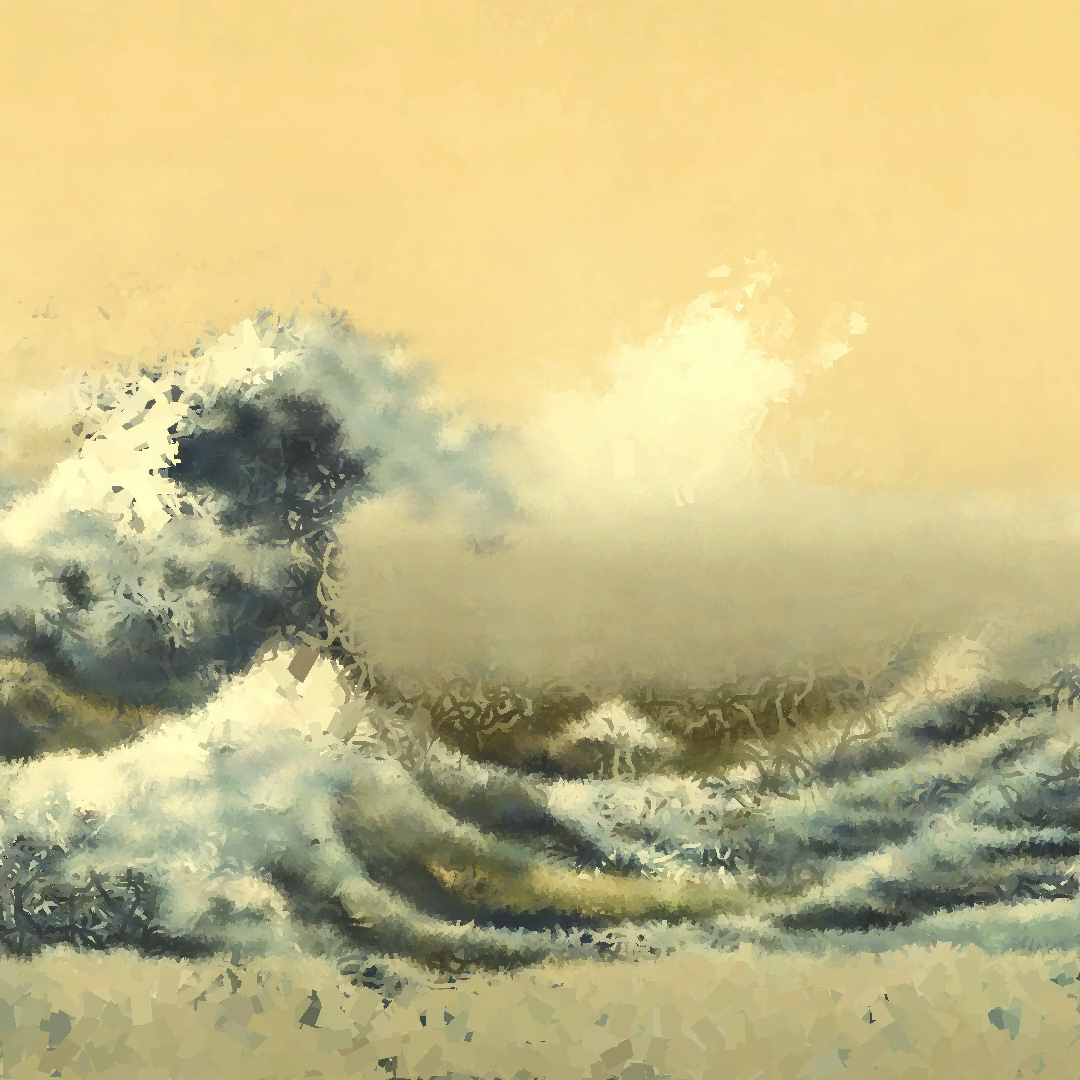
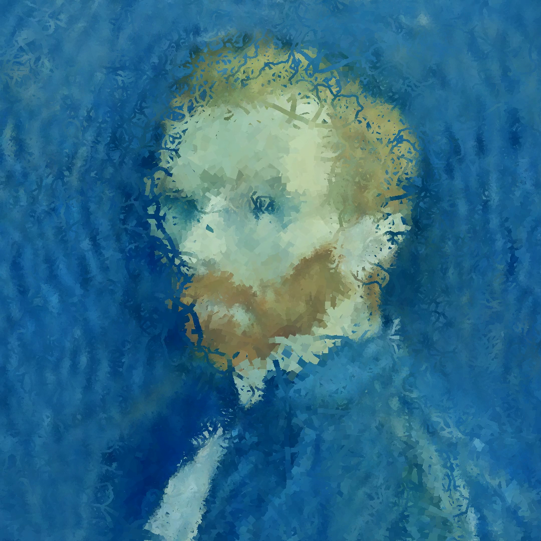
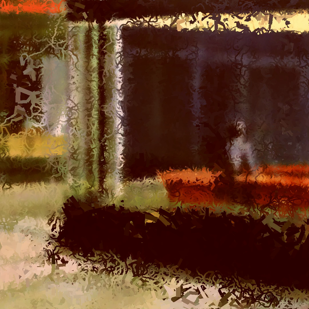
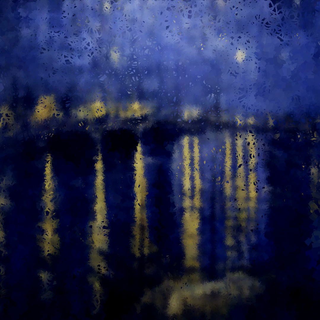
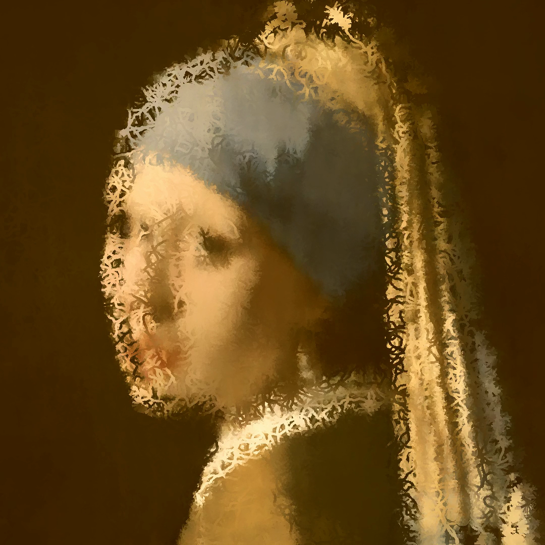
Figure 5.4. Late frames from five final videos. Each frame is produced by the same workflow, but the reference image, audio features, zoom behavior, and rendering settings lead to different color ranges, stroke textures, and image structures.
How to Read a Result: Do not judge only by the emotional label. Look for visible evidence: color range, readable image structure, stroke density, scale, and how much the canvas has accumulated. These are the signs that connect the result back to the method.
What the Results Show
The results show that the system can turn a still reference image into a moving painting without simply playing the original image as a slideshow. The reference image remains recognizable, but it is rebuilt from many small strokes. This is important because the project is not only about image generation. It is about a painting process that unfolds with music.
The results also show the difference between color learning and painting. The neural network gives the painter a color rule. It helps the system choose colors that belong to the reference image at each location and music frame. The random walk gives the result its visible motion and texture. Because the canvas is not cleared between frames, marks accumulate and the image becomes denser as the video continues.
A single still frame cannot show everything. The final video also contains zoom changes, changes in walker speed, changes in stroke width, and changes in opacity. Those time-based changes are connected to the music features. Therefore, the most complete way to read the output is to compare both a still frame and the moving video: the frame shows the accumulated painting, while the video shows how the painting arrives there.
The five moving paintings can be watched in Chapter 11. The still frames here show accumulated marks; the videos show how those marks develop with the music.
Summary
The painter connects a learned color rule, random paths, music intensity, and local image-region controls. The network supplies stroke color, while walkers create the path and deposit marks. The canvas carries its history from one frame to the next.
training checkpoint notebook integration RW_Painter rendering frames final video.
Chapter 11 explores how choices of image, music, visual scale, and rendering style turn this shared process into distinct artistic works.
Appendix
File Map
The main chapter explains the ideas in a teaching order. The program itself is organized by files. Table 5.1 gives a compact map for review.
| File | Role in the workflow |
|---|---|
neural_network_music.py | Builds Mel spectrograms, computes zoom levels, defines XYSpecNet, trains the neural color model, saves checkpoints, and contains the video-combining helper. |
random_walk_image.ipynb | Loads a checkpoint, chooses the audio clip and render settings, rebuilds the model, prepares music features for the selected clip, creates RW_Painter, and starts rendering. |
RWraw.py | Defines RW_Painter. This class manages walkers, predicts colors with the trained model, uses image-region information, draws strokes, and saves numbered PNG frames. |
Table 5.1. Main source files used by the Inner Landscapes workflow.
Core Settings
The following settings are useful when checking whether an explanation, figure, or result matches the implementation.
| Setting | Value or meaning |
|---|---|
| Training image grid | locations |
| Rendering canvas | pixels in the notebook render setup |
| Target frame rate | frames per second for music features and video frames |
| Neural-network music features | Mel values per music frame |
| Zoom-decision spectrogram | Mel values per music frame |
| Fourier coordinate frequencies | Most emotions use ; Nostalgia also uses |
| Model output | Three RGB values between and |
| Final frame format | Numbered PNG files such as 000000.png, 000001.png, and so on |
| Final video step | The saved frames are combined with the selected audio clip |
Table 5.2. Core settings used throughout the chapter.
Reproduction Checklist
To reproduce the project, follow the same order as the real workflow.
-
Prepare the reference image and audio file for each emotion.
-
Run the training script so the program can build music features, select zoom targets, train
XYSpecNet, and save a checkpoint. -
Confirm that the checkpoint exists before rendering.
-
Open the notebook and choose the emotion, audio segment, and render settings.
-
Let the notebook load the checkpoint, rebuild the model, normalize the clip’s music features with the saved values, and create
RW_Painter. -
Render the numbered PNG frames.
-
Combine the frames with the audio clip to create the final video.
Common Problems to Check
Table 5.3. Practical checks for reproducing the workflow.
| Problem | What to check |
|---|---|
| The notebook skips an emotion | The checkpoint path may be missing. Run the training script for that emotion first. |
| The colors look wrong | Check that the notebook uses the saved spec_min and spec_max from the checkpoint when normalizing the rendering clip. |
| The output does not respond clearly to music | Check that the selected audio segment has enough changing spectrogram energy and that the zoom levels are being sliced for the same time segment. |
| The painting looks too empty early in the video | Remember that the canvas accumulates over time. Early frames naturally contain fewer marks than late frames. |
| The final video is missing audio or does not export | Check that the numbered PNG frames were saved and that the video-combining command can access the audio clip. |